library(stacked)
library(data.table)

# Load the ACS microdata sample
data(acs_micro)

# Structure of the data
str(acs_micro)
#> Classes 'data.table' and 'data.frame':   69820 obs. of  8 variables:
#>  $ state     : chr  "AL" "AL" "AL" "AL" ...
#>  $ year      : int  2008 2008 2008 2008 2008 2008 2008 2008 2008 2008 ...
#>  $ perwt     : int  116 121 93 135 94 242 180 215 250 83 ...
#>  $ statefip  : int  1 1 1 1 1 1 1 1 1 1 ...
#>  $ adopt_year: int  NA NA NA NA NA NA NA NA NA NA ...
#>  $ uninsured : int  0 1 1 0 0 0 1 0 0 0 ...
#>  $ female    : int  1 0 0 1 0 1 1 1 0 1 ...
#>  $ age       : int  19 46 49 20 23 51 46 35 20 26 ...
#>  - attr(*, ".internal.selfref")=<externalptr>

# Sample sizes by year
acs_micro[, .N, by = year][order(year)]
#>     year    N
#>  1: 2008 4980
#>  2: 2009 5005
#>  3: 2010 5048
#>  4: 2011 5099
#>  5: 2012 5080
#>  6: 2013 5110
#>  7: 2014 5065
#>  8: 2015 5065
#>  9: 2016 5039
#> 10: 2017 5083
#> 11: 2018 5078
#> 12: 2019 5049
#> 13: 2020 4112
#> 14: 2021 5007

# Adoption year distribution
acs_micro[, .(n_obs = .N), by = adopt_year][order(adopt_year)]
#>    adopt_year n_obs
#> 1:       2014 39245
#> 2:       2015  4469
#> 3:       2016  1175
#> 4:       2019  2177
#> 5:       2020  1393
#> 6:       2021  2173
#> 7: NA 19188Working with Repeated Cross-Section Data
Using stacked with survey microdata — RCS Q-weights, survey weights, and propensity-score weighting — in R and Stata.
Overview
This vignette demonstrates how to use the stacked package with repeated cross-section (RCS) data. Unlike panel data where the same units are observed over time, RCS data consists of independent samples drawn at each time period. Common examples include:
- American Community Survey (ACS) microdata
- Current Population Survey (CPS)
- Behavioral Risk Factor Surveillance System (BRFSS)
- Any survey with fresh random samples each wave
The package handles RCS data through the data_type = "repeated_cross_section" argument in build_stack() and add_pscore_weights().
When to Use Repeated Cross-Section Mode
Use data_type = "repeated_cross_section" when:
- Different individuals appear in each time period: The data contains independent samples, not the same people tracked over time
- Sample sizes vary across time periods: Unlike balanced panels, RCS typically has different numbers of observations per period
- Survey weights are important: RCS data often comes from complex survey designs with sampling weights
The key difference from panel data is that Q-weights in RCS mode include an additional event-time level adjustment to account for varying sample compositions across time periods.
The Dataset: ACS Microdata
We’ll use the acs_micro dataset, which is a stratified 0.3% sample of the American Community Survey for 2008-2021. This dataset contains individual-level records with covariates suitable for propensity score estimation.
* Load the bundled ACS microdata sample
stacked use acs_micro, clear

* Sample sizes by year
tabulate year

* Adoption year distribution
tabulate adopt_year, missing
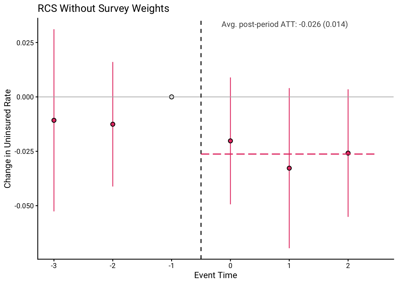
Scenario 1: RCS Without Survey Weights
In the simplest case, you might want to ignore survey weights (e.g., for exploratory analysis or when weights are unavailable). This still uses the RCS-specific Q-weight formula.
# Build stacked dataset (RCS mode, no weights)
stack1 <- build_stack(
  data = acs_micro,
  time_var = "year",
  unit_var = "state",
  adopt_var = "adopt_year",
  kappa_pre = 3,
  kappa_post = 2,
  data_type = "repeated_cross_section"  # Key difference from panel
)

# Examine the structure
head(stack1[, .(state, year, sub_exp, event_time, treat, q_weight)])
#>    state year sub_exp event_time treat q_weight
#> 1:    AL 2011    2014         -3     0 3.161019
#> 2:    AL 2011    2014         -3     0 3.161019
#> 3:    AL 2011    2014         -3     0 3.161019
#> 4:    AL 2011    2014         -3     0 3.161019
#> 5:    AL 2011    2014         -3     0 3.161019
#> 6:    AL 2011    2014         -3     0 3.161019

# Note: q_weight now accounts for varying sample sizes across event times
stack1[, .(
  mean_q_weight = mean(q_weight),
  n_obs = .N
), by = .(sub_exp, event_time)][order(sub_exp, event_time)]
#>     sub_exp event_time mean_q_weight n_obs
#>  1:    2014         -3     1.8374220  4681
#>  2:    2014         -2     1.8443355  4663
#>  3:    2014         -1     1.8367850  4694
#>  4:    2014          0     1.8437343  4655
#>  5:    2014          1     1.7635908  4658
#>  6:    2014          2     1.8489741  4640
#>  7:    2015         -3     0.4547448  2139
#>  8:    2015         -2     0.4525847  2149
#>  9:    2015         -1     0.4564898  2136
#> 10:    2015          0     0.4544099  2136
#> 11:    2015          1     0.4367780  2127
#> 12:    2015          2     0.4502280  2155
#> 13:    2016         -3     0.1349442  1911
#> 14:    2016         -2     0.1358553  1898
#> 15:    2016         -1     0.1359836  1901
#> 16:    2016          0     0.1357210  1896
#> 17:    2016          1     0.1282145  1921
#> 18:    2016          2     0.1336937  1924
#> 19:    2019         -3     0.2940670  1559
#> 20:    2019         -2     0.2903140  1579
#> 21:    2019         -1     0.2901289  1584
#> 22:    2019          0     0.2893550  1581
#> 23:    2019          1     0.3902557  1122
#> 24:    2019          2     0.2959819  1545
#>     sub_exp event_time mean_q_weight n_obs
* Build stacked dataset in RCS mode (no survey weights)
stacked use acs_micro, clear
stacked build, time(year) unit(statefip) adopt(adopt_year) ///
kpre(3) kpost(2) datatype(rcs)
list statefip year sub_exp event_time treat q_weight in 1/6Fitting the Event Study
# Fit event study using stackreg
model1 <- stackreg(
  stack_data = stack1,
  outcome_var = "uninsured",
  cluster_var = "state"
)

# Create event study plot
stack_plot(
  model1,
  title = "RCS Without Survey Weights",
  ylab = "Change in Uninsured Rate"
)
* Fit the event study and plot the coefficients
stacked reg uninsured, cluster(statefip)
stacked plot, title("RCS Without Survey Weights")
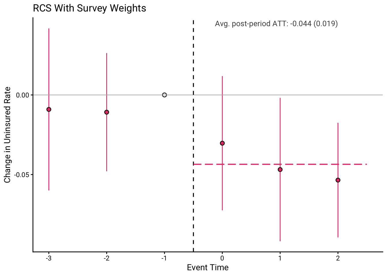
Scenario 2: RCS With Survey Weights
When using complex survey data, you should incorporate the survey sampling weights. The weight_var parameter tells build_stack() to use these weights in the Q-weight calculations.
# Build stacked dataset with survey weights
stack2 <- build_stack(
  data = acs_micro,
  time_var = "year",
  unit_var = "state",
  adopt_var = "adopt_year",
  kappa_pre = 3,
  kappa_post = 2,
  weight_var = "perwt",  # ACS person weight
  data_type = "repeated_cross_section"
)

# Compare Q-weight distributions between scenarios
cat("Q-weight summary - Without survey weights:\n")
#> Q-weight summary - Without survey weights:
print(summary(stack1$q_weight))
#>    Min. 1st Qu.  Median    Mean 3rd Qu.    Max.
#> 0.08814 0.21737 0.98388 1.00000 1.00297 3.17183

cat("\nQ-weight summary - With survey weights:\n")
#>
#> Q-weight summary - With survey weights:
print(summary(stack2$q_weight))
#>     Min.  1st Qu.   Median     Mean  3rd Qu.     Max.
#>    0.098   16.606   47.650  108.247  122.818 4058.603

# The distributions differ because survey weights affect Q-weight calculations
* Build stacked dataset with the ACS person weight
stacked use acs_micro, clear
stacked build, time(year) unit(statefip) adopt(adopt_year) ///
kpre(3) kpost(2) datatype(rcs) weightvar(perwt)
summarize q_weightFitting the Event Study with Survey Weights
# Fit event study using stackreg
model2 <- stackreg(
  stack_data = stack2,
  outcome_var = "uninsured",
  cluster_var = "state"
)

# Create event study plot
stack_plot(
  model2,
  title = "RCS With Survey Weights",
  ylab = "Change in Uninsured Rate"
)
* Fit the event study and plot the coefficients
stacked reg uninsured, cluster(statefip)
stacked plot, title("RCS With Survey Weights")
Scenario 3: RCS With Propensity Score Weights
For the most robust analysis, you can combine RCS handling with propensity score weighting. This addresses both:
- The RCS structure (through Q-weights with event-time adjustment)
- Covariate imbalance (through inverse propensity weighting)
Step 1: Estimate Propensity Scores
# Use the survey-weighted stack from Scenario 2
stack3 <- copy(stack2)

# Estimate propensity scores using available covariates
# We'll estimate within sub_exp x event_time cells for flexibility
stack3[, phat := {
  if (length(unique(treat)) == 2 && sum(treat) >= 5 && sum(1-treat) >= 5) {
    # Fit logistic model with age and sex
    fit <- glm(treat ~ female + age, family = binomial, data = .SD)
    predict(fit, type = "response")
  } else {
    # If insufficient variation, use overall treatment rate
    mean(treat)
  }
}, by = .(sub_exp, event_time)]

# Check propensity score distribution
summary(stack3$phat)
#>    Min. 1st Qu.  Median    Mean 3rd Qu.    Max.
#> 0.02715 0.09887 0.15851 0.33418 0.61111 0.63317
Step 2: Trim Extreme Propensity Scores
Before calling add_pscore_weights(), apply your preferred trimming strategy. The function requires propensity scores strictly between 0 and 1.
# Check for boundary values
cat("Observations at boundaries before trimming:\n")
#> Observations at boundaries before trimming:
cat("  p = 0:", sum(stack3$phat == 0), "\n")
#>   p = 0: 0
cat("  p = 1:", sum(stack3$phat == 1), "\n")
#>   p = 1: 0
cat("  p < 0.01:", sum(stack3$phat < 0.01), "\n")
#>   p < 0.01: 0
cat("  p > 0.99:", sum(stack3$phat > 0.99), "\n")
#>   p > 0.99: 0

# Apply trimming - remove observations with extreme propensity scores
# This is the recommended approach for maintaining sample integrity
stack3_trimmed <- stack3[phat > 0.01 & phat < 0.99]

cat("\nRows before trimming:", nrow(stack3), "\n")
#>
#> Rows before trimming: 61254
cat("Rows after trimming:", nrow(stack3_trimmed), "\n")
#> Rows after trimming: 61254
cat("Percent retained:", round(100 * nrow(stack3_trimmed) / nrow(stack3), 1), "%\n")
#> Percent retained: 100 %

# Alternative: Winsorize instead of drop
# stack3[, phat := pmin(pmax(phat, 0.01), 0.99)]
Step 3: Add Propensity Score Weights
# Add propensity score weights
# Q-weights are recomputed from the trimmed sample
stack3_ps <- add_pscore_weights(
  stack_data = stack3_trimmed,
  pscore_var = "phat",
  weight_var = "perwt",
  data_type = "repeated_cross_section"
)

# Compare original Q-weights to propensity-adjusted Q-weights
head(stack3_ps[, .(state, year, treat, phat, q_weight, q_weight_ps)])
#>    state year treat      phat q_weight q_weight_ps
#> 1:    AL 2011     0 0.6151815 672.2259   341.29894
#> 2:    AL 2011     0 0.6134865 107.3037    54.09129
#> 3:    AL 2011     0 0.6151815 729.0337   370.14110
#> 4:    AL 2011     0 0.6151556 400.8107   203.47526
#> 5:    AL 2011     0 0.6131472 208.2954   104.85060
#> 6:    AL 2011     0 0.6080442 261.9472   129.05780

# Weight distributions by treatment status
cat("\nQ-weight distribution by treatment:\n")
#>
#> Q-weight distribution by treatment:
stack3_ps[, .(
  mean_qw = mean(q_weight),
  mean_qw_ps = mean(q_weight_ps),
  sd_qw_ps = sd(q_weight_ps)
), by = treat]
#>    treat  mean_qw mean_qw_ps  sd_qw_ps
#> 1:     0 109.1748   54.09567 102.12795
#> 2:     1 106.3992  106.39917  86.72463
* Add propensity-score-adjusted weights (RCS mode, survey weights)
* phat must already be in the data, strictly inside (0, 1)
stacked pscore, pscore(phat) weightvar(perwt) datatype(rcs)
list statefip year treat phat q_weight q_weight_ps in 1/6Step 4: Fit Event Study with Propensity Score Weights
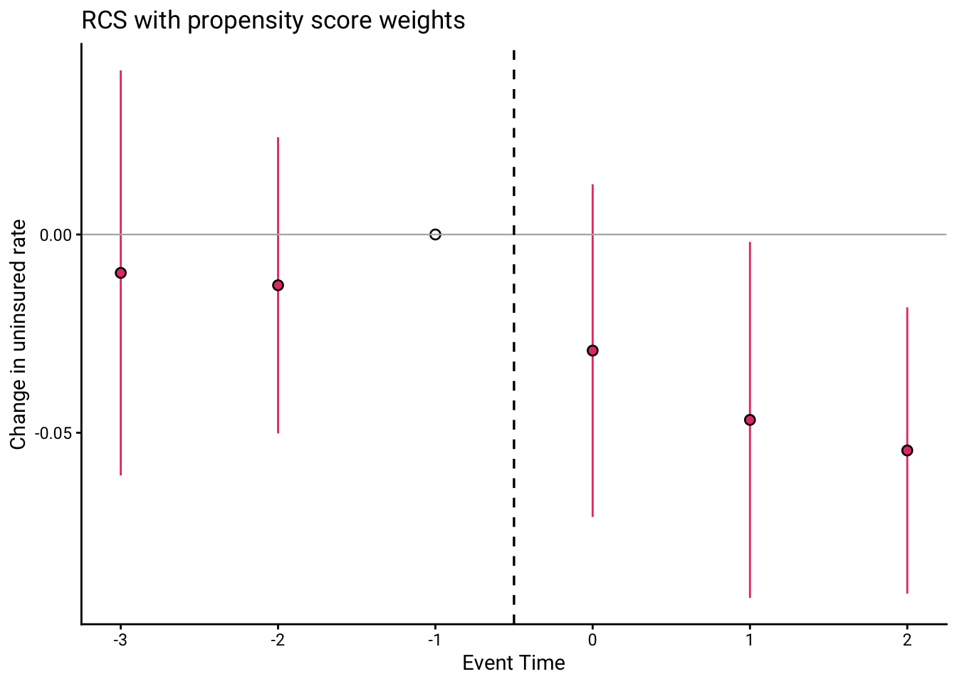
For propensity score weights we fit with the q_weight_ps column. Because this is a custom weight column, we call fixest::feols() directly instead of stackreg() (which always uses q_weight). The resulting model still has the standard treat:i(event_time) structure, so stack_plot() reads it and draws the event study in the house style — no manual coefficient extraction needed.
library(fixest)

# Fit the saturated regression with propensity-score-adjusted weights
model3 <- feols(
  uninsured ~ treat * i(event_time, ref = -1),
  data = stack3_ps,
  weights = ~q_weight_ps,
  cluster = ~state
)

# stack_plot() extracts the treat x event_time coefficients and plots them
stack_plot(
  model3,
  title = "RCS with propensity score weights",
  ylab = "Change in uninsured rate"
)
* Propensity-score-adjusted Q-weights, then the event study + coefficient plot
stacked pscore, pscore(phat) weightvar(perwt) datatype(rcs)
stacked reg uninsured, cluster(state) ref(-1)
stacked plot, title("RCS with propensity score weights")
Checking Covariate Balance
After applying propensity score weights, verify that covariate balance improved:
# Calculate balance statistics
balance_stats <- stack3_ps[, .(
  # Unweighted means
  female_treat_raw = mean(female[treat == 1]),
  female_control_raw = mean(female[treat == 0]),
  age_treat_raw = mean(age[treat == 1]),
  age_control_raw = mean(age[treat == 0]),

  # Survey-weighted means (original q_weight)
  female_treat_sw = weighted.mean(female[treat == 1], q_weight[treat == 1]),
  female_control_sw = weighted.mean(female[treat == 0], q_weight[treat == 0]),
  age_treat_sw = weighted.mean(age[treat == 1], q_weight[treat == 1]),
  age_control_sw = weighted.mean(age[treat == 0], q_weight[treat == 0]),

  # PS-weighted means
  female_treat_ps = weighted.mean(female[treat == 1], q_weight_ps[treat == 1]),
  female_control_ps = weighted.mean(female[treat == 0], q_weight_ps[treat == 0]),
  age_treat_ps = weighted.mean(age[treat == 1], q_weight_ps[treat == 1]),
  age_control_ps = weighted.mean(age[treat == 0], q_weight_ps[treat == 0])
)]

# Display balance comparison
cat("Female covariate balance:\n")
#> Female covariate balance:
cat("  Raw difference:",
    round(balance_stats$female_treat_raw - balance_stats$female_control_raw, 4), "\n")
#>   Raw difference: 0.0036
cat("  Survey-weighted difference:",
    round(balance_stats$female_treat_sw - balance_stats$female_control_sw, 4), "\n")
#>   Survey-weighted difference: -0.0015
cat("  PS-weighted difference:",
    round(balance_stats$female_treat_ps - balance_stats$female_control_ps, 4), "\n")
#>   PS-weighted difference: -0.0039

cat("\nAge covariate balance:\n")
#>
#> Age covariate balance:
cat("  Raw difference:",
    round(balance_stats$age_treat_raw - balance_stats$age_control_raw, 2), "years\n")
#>   Raw difference: 0.31 years
cat("  Survey-weighted difference:",
    round(balance_stats$age_treat_sw - balance_stats$age_control_sw, 2), "years\n")
#>   Survey-weighted difference: 0.35 years
cat("  PS-weighted difference:",
    round(balance_stats$age_treat_ps - balance_stats$age_control_ps, 2), "years\n")
#>   PS-weighted difference: 0.1 years
Comparison: Panel vs RCS Modes
To illustrate the difference between panel and RCS modes, compare the Q-weights:
# Build with panel mode for comparison (inappropriate for this data, but illustrative)
stack_panel <- build_stack(
  data = acs_micro,
  time_var = "year",
  unit_var = "state",
  adopt_var = "adopt_year",
  kappa_pre = 3,
  kappa_post = 2,
  weight_var = "perwt",
  data_type = "panel"  # Wrong for RCS data, but for comparison
)

# Compare Q-weight distributions
cat("Q-weight summary - Panel mode:\n")
#> Q-weight summary - Panel mode:
print(summary(stack_panel$q_weight))
#>     Min.  1st Qu.   Median     Mean  3rd Qu.     Max.
#>    0.097   16.635   47.631  108.247  123.000 4077.804

cat("\nQ-weight summary - RCS mode:\n")
#>
#> Q-weight summary - RCS mode:
print(summary(stack2$q_weight))
#>     Min.  1st Qu.   Median     Mean  3rd Qu.     Max.
#>    0.098   16.606   47.650  108.247  122.818 4058.603

# The differences arise because RCS mode accounts for varying sample sizes
# across event times within each sub-experiment
* Build with panel mode for comparison (inappropriate here, illustrative only)
stacked use acs_micro, clear
stacked build, time(year) unit(statefip) adopt(adopt_year) ///
kpre(3) kpost(2) weightvar(perwt) datatype(panel)
summarize q_weightBest Practices for RCS Analysis
Always use
data_type = "repeated_cross_section"for survey data with independent samples at each time periodInclude survey weights via
weight_varto properly account for complex survey designsConsider propensity score weighting when treated and control groups differ systematically on observed characteristics
Apply user trimming before
add_pscore_weights()- choose bounds appropriate for your application (e.g., 0.01/0.99 or 0.05/0.95)Check covariate balance before and after applying propensity score weights to verify improvement
Cluster standard errors appropriately - typically at the unit (state) level for geographic policy evaluations
Summary
The stacked package provides comprehensive support for repeated cross-section data through:
data_type = "repeated_cross_section"inbuild_stack()for correct Q-weight formulasweight_varparameter for incorporating survey sampling weightsadd_pscore_weights()withdata_type = "repeated_cross_section"for propensity score weighting- User-controlled trimming for handling extreme propensity scores
This flexibility allows researchers to implement the stacked DID method with the same rigor for RCS data as for panel data.
References
Wing, C., Hollingsworth, A., & Freedman, S. (2024). Stacked Difference-in-Differences. Working Paper.