install.packages(c("DBI", "duckdb"))Larger-than-Memory Data with duck = TRUE
Running the whole stacked workflow inside DuckDB — build, weight, and estimate against parquet files that never enter memory — in R and Stata.
Overview
The core stacked functions can run against data that never enters R memory. Setting duck = TRUE pushes the heavy work — building the stacked dataset, computing Q-weights, counting observations for the kappa trade-off table, and even the weighted event-study regression — into DuckDB, an embedded analytical database that reads parquet/csv files directly and spills to disk when data exceeds RAM.
Three functions accept duck = TRUE (or a duck input) directly:
| Function | duck behavior |
|---|---|
kappa_trade_offs(..., duck = TRUE) |
Counts computed in DuckDB; returns the usual small data.table |
build_stack(..., duck = TRUE) |
Stack built inside DuckDB; returns a stack_duck handle, not a data.table |
stackreg(stack_duck, ...) |
Detects the handle automatically; exact weighted regression via SQL compression |
stack_levels() also accepts a stack_duck handle.
The results are numerically identical to the in-memory path: the package’s test suite verifies counts exactly and estimates, standard errors, and full variance matrices to about 1e-8 (float-summation order) on all bundled datasets.
In Stata, the same backend is reached with parquet() (for stacked build and stacked kappa) and the duck option (for stacked reg and stacked levels); the stacked dataset is created inside DuckDB and never enters Stata memory.
Setup
duck = TRUE needs two extra packages (both in Suggests):
* Fetch DuckDB's self-contained JDBC driver once (~75 MB, into PERSONAL)
stacked duckconnect, downloadlibrary(stacked)
library(data.table)Three ways to supply data
1. A file path or glob (the larger-than-memory case). Point directly at parquet or csv files; DuckDB scans them without loading:
kt <- kappa_trade_offs("panel/*.parquet", "year", "state", "adopt_year",
                       duck = TRUE)
stack <- build_stack("panel/*.parquet", "year", "state", "adopt_year",
                     kappa_pre = 3, kappa_post = 2, duck = TRUE)
* Point kappa/build at parquet (or csv) files or a glob
stacked duckconnect
stacked kappa, parquet("panel/*.parquet") time(year) unit(state) ///
adopt(adopt_year)
stacked build, parquet("panel/*.parquet") time(year) unit(state) ///
adopt(adopt_year) kpre(3) kpost(2)2. A data.frame. Handy for testing the duck path against the in-memory path on identical input — the data is registered with DuckDB as a view, not copied:
data(medicaid)
kt <- kappa_trade_offs(medicaid, "year", "state", "adopt_year",
                       kappa_pre_range = 1:3, kappa_post_range = 1:3,
                       duck = TRUE)
kt
#>    kappa_pre kappa_post n_sub_exp n_unidentified_sub_exp n_event_times n_obs
#> 1:         1          1         5                      0             3   354
#> 2:         1          2         4                      0             4   400
#> 3:         1          3         3                      0             5   425
#> 4:         2          1         5                      0             4   472
#> 5:         2          2         4                      0             5   500
#> 6:         2          3         3                      0             6   510
#> 7:         3          1         5                      0             5   590
#> 8:         3          2         4                      0             6   600
#> 9:         3          3         3                      0             7   595
#>    total_treated_obs total_control_obs avg_treated_per_period
#> 1:               114               240                     38
#> 2:               140               260                     35
#> 3:               165               260                     33
#> 4:               152               320                     38
#> 5:               175               325                     35
#> 6:               198               312                     33
#> 7:               190               400                     38
#> 8:               210               390                     35
#> 9:               231               364                     33
#>    avg_control_per_period sd_treated_per_period sd_control_per_period
#> 1:                     80                     0                     0
#> 2:                     65                     0                     0
#> 3:                     52                     0                     0
#> 4:                     80                     0                     0
#> 5:                     65                     0                     0
#> 6:                     52                     0                     0
#> 7:                     80                     0                     0
#> 8:                     65                     0                     0
#> 9:                     52                     0                     0
#>              adoption_times_str
#> 1: 2014, 2015, 2016, 2019, 2020
#> 2:       2014, 2015, 2016, 2019
#> 3:             2014, 2015, 2016
#> 4: 2014, 2015, 2016, 2019, 2020
#> 5:       2014, 2015, 2016, 2019
#> 6:             2014, 2015, 2016
#> 7: 2014, 2015, 2016, 2019, 2020
#> 8:       2014, 2015, 2016, 2019
#> 9:             2014, 2015, 2016
* In Stata the duck path always reads a parquet/csv file; export once,
* then point parquet() at it
stacked use medicaid, clear
export delimited using "medicaid.csv", replace
stacked kappa, parquet("medicaid.csv") time(year) unit(state) ///
adopt(adopt_year) kpre(1/3) kpost(1/3)3. Your own DuckDB connection. If the data already lives in a DuckDB database, wrap the connection and table name with duck_src(). The package never closes a connection you own:
con <- DBI::dbConnect(duckdb::duckdb("my_database.duckdb"))
src <- duck_src(con, table = "panel")
stack <- build_stack(src, "year", "state", "adopt_year",
                     kappa_pre = 3, kappa_post = 2,
                     duck_table_name = "my_stack")  # persists in your DB
duck_src() also takes duck_options for package-opened connections, e.g. duck_src("panel/*.parquet", duck_options = list(memory_limit = "8GB", threads = 4)).
Step 1: choose kappas
kappa_trade_offs() works exactly as usual — only the computation moves into DuckDB. On a 60 million row panel this takes seconds:
kappa_trade_offs(medicaid, "year", "state", "adopt_year",
                 kappa_pre_range = 2:3, kappa_post_range = 1:2,
                 duck = TRUE)
#>    kappa_pre kappa_post n_sub_exp n_unidentified_sub_exp n_event_times n_obs
#> 1:         2          1         5                      0             4   472
#> 2:         2          2         4                      0             5   500
#> 3:         3          1         5                      0             5   590
#> 4:         3          2         4                      0             6   600
#>    total_treated_obs total_control_obs avg_treated_per_period
#> 1:               152               320                     38
#> 2:               175               325                     35
#> 3:               190               400                     38
#> 4:               210               390                     35
#>    avg_control_per_period sd_treated_per_period sd_control_per_period
#> 1:                     80                     0                     0
#> 2:                     65                     0                     0
#> 3:                     80                     0                     0
#> 4:                     65                     0                     0
#>              adoption_times_str
#> 1: 2014, 2015, 2016, 2019, 2020
#> 2:       2014, 2015, 2016, 2019
#> 3: 2014, 2015, 2016, 2019, 2020
#> 4:       2014, 2015, 2016, 2019
stacked kappa, parquet("medicaid.parquet") time(year) unit(state) ///
adopt(adopt_year) kpre(2/3) kpost(1/2)Step 2: build the stack
With duck = TRUE, build_stack() returns a stack_duck handle instead of a data.table. The stacked rows stay inside DuckDB:
stack <- build_stack(medicaid, "year", "state", "adopt_year",
                     kappa_pre = 3, kappa_post = 2, duck = TRUE)
stack
#> <stack_duck> DuckDB-backed stacked dataset
#>   table:      stacked_stack_1 (package-owned connection)
#>   rows:       600  (treated 210 / control 390)
#>   event time: -3 to 2
#>   params:     kappa_pre=3, kappa_post=2, control_type=both
#>   first rows:
#>   state statefip year adopt_year uninsured sub_exp event_time treat post
#> 1    TX       48 2018         NA 0.2551008    2016          2     0    1
#> 2    NE       31 2014       2020 0.1384460    2016         -2     0    0
#> 3    MO       29 2018       2021 0.1468473    2016          2     0    1
#> 4    OK       40 2018       2021 0.2122405    2016          2     0    1
#> 5    LA       22 2018       2016 0.1319689    2016          2     1    1
#>    q_weight
#> 1 0.2063492
#> 2 0.2063492
#> 3 0.2063492
#> 4 0.2063492
#> 5 1.0000000
* The stacked dataset is created inside DuckDB, not loaded into Stata
stacked build, parquet("medicaid.parquet") time(year) unit(state) ///
adopt(adopt_year) kpre(3) kpost(2)The handle knows its dimensions without materializing anything (stack$n_obs, stack$n_treated, stack$event_times), and there are a few utilities:
head(duck_collect(stack, n = 3))          # peek at a few rows
#>    state statefip year adopt_year uninsured sub_exp event_time treat post
#> 1:    TX       48 2018         NA 0.2551008    2016          2     0    1
#> 2:    NE       31 2014       2020 0.1384460    2016         -2     0    0
#> 3:    MO       29 2018       2021 0.1468473    2016          2     0    1
#>     q_weight
#> 1: 0.2063492
#> 2: 0.2063492
#> 3: 0.2063492
full_dt <- duck_collect(stack) # materialize everything (careful!)
duck_write_parquet(stack, "stack.parquet") # export without touching R memory
duck_disconnect(stack) # explicit cleanup (also automatic on GC)Step 3: estimate
stackreg() recognizes the handle automatically — no new arguments:
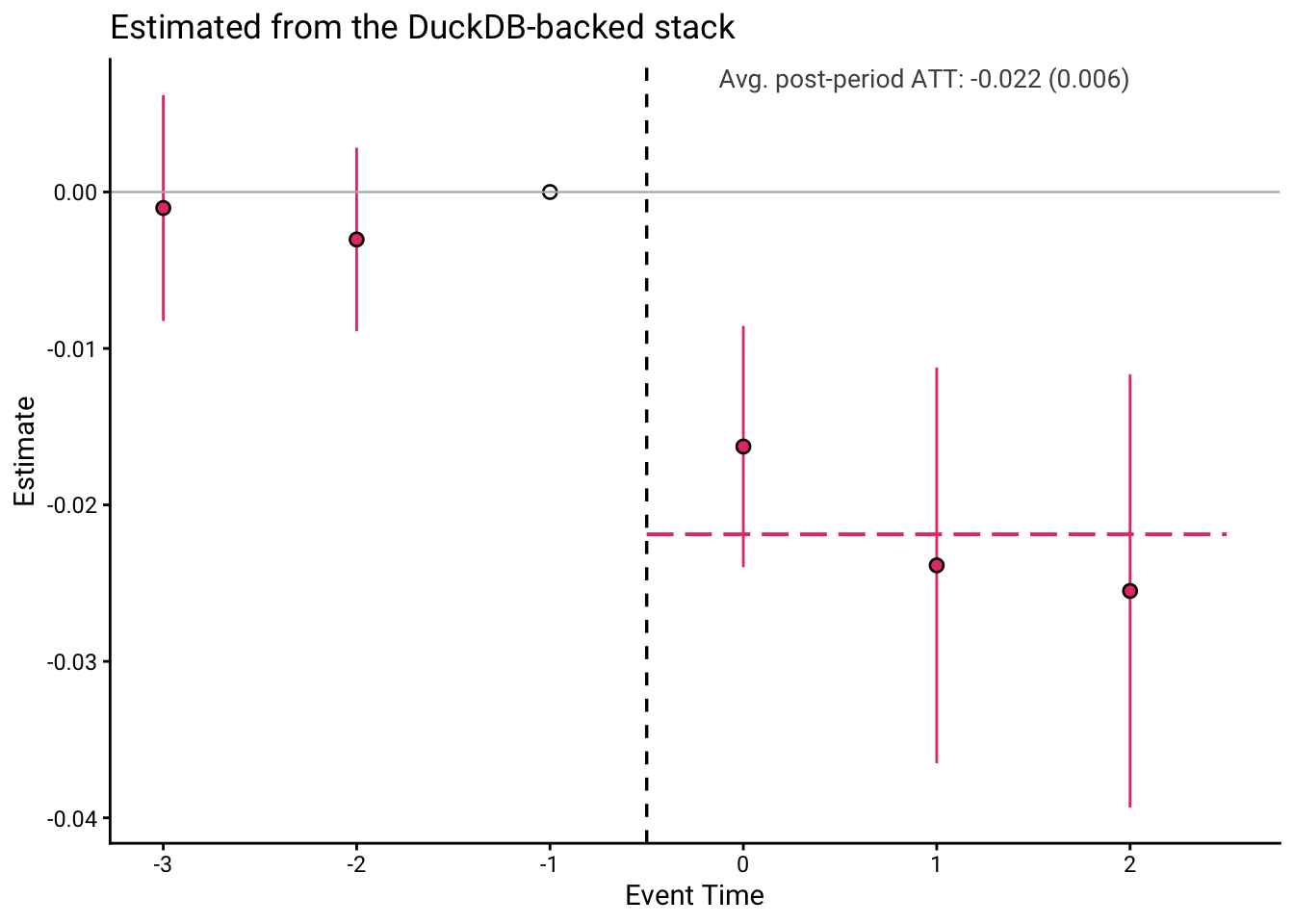
model <- stackreg(stack, "uninsured", cluster_var = "state")
attr(model, "avg_post_att")
#> $estimate
#> [1] -0.02187775
#>
#> $se
#> [1] 0.005628133
#>
#> $ci_lower
#> [1] -0.03290869
#>
#> $ci_upper
#> [1] -0.01084681
#>
#> $n_periods
#> [1] 3
#>
#> $conf_level
#> [1] 0.95
* Estimate from the exact cell compression inside DuckDB
stacked reg uninsured, duck cluster(state)Everything downstream works unchanged, because stackreg() returns a regular fixest object:
stack_coefs(model)
#>    event_time     estimate          se     ci_lower     ci_upper
#> 1:         -3 -0.001022172 0.003682642 -0.008240017  0.006195674
#> 2:         -2 -0.003034560 0.002993349 -0.008901416  0.002832296
#> 3:         -1  0.000000000          NA           NA           NA
#> 4:          0 -0.016269503 0.003933884 -0.023979774 -0.008559231
#> 5:          1 -0.023863697 0.006453761 -0.036512836 -0.011214558
#> 6:          2 -0.025500057 0.007066243 -0.039349639 -0.011650476
if (requireNamespace("ggplot2", quietly = TRUE)) {
  stack_plot(model, title = "Estimated from the DuckDB-backed stack")
}
Per-timing-group estimation works at full speed too – adding sub_exp to the cell grouping gives per-cohort compression for free:
groups <- stackreg(stack, "uninsured", cluster_var = "state",
                   by_group = TRUE)
groups
#> <stackreg_groups> event study by timing group (4 cohorts)
#>
#>    sub_exp        att         se    weight
#> 1:    2014 -0.0215517 0.00650243 0.8000000
#> 2:    2015 -0.0158562 0.00521068 0.0857143
#> 3:    2016 -0.0421334 0.00414854 0.0571429
#> 4:    2019 -0.0152191 0.00394367 0.0571429
#>
#> pooled: -0.0218778 (se 0.00562813);  weighted sum of cohort ATTs: -0.0218778
* Per-cohort estimates and weights, at full duck speed
stacked reg uninsured, duck cluster(state) bygroup
matrix list r(group_att)stack_levels() runs as a single grouped query:
stack_levels(stack, "uninsured")
#>    event_time treat_mean_uninsured control_mean_uninsured
#> 1:         -3           0.18461237              0.2268165
#> 2:         -2           0.17835218              0.2225687
#> 3:         -1           0.17435925              0.2155412
#> 4:          0           0.13272761              0.1901791
#> 5:          1           0.10582017              0.1708659
#> 6:          2           0.09608882              0.1627709
stacked levels uninsured, duck
matrix list r(levels)Population weights, including time-varying ones
All panel weight_type options work with duck = TRUE, exactly as they do in memory — the sub-experiment shares become window functions over the weighted population sums, so nothing changes in how you call the functions. A typical use: units are counties of very different sizes and you want a person-weighted ATT, with weights that track each county’s population over the event window:
# medicaid with a synthetic time-varying population, for illustration
md <- data.table::as.data.table(medicaid)
md[, pop := 1e5 * (1 + (statefip %% 7) / 10) * (1 + 0.02 * (year - 2008))]

stack_pop <- build_stack(md, "year", "state", "adopt_year",
                         kappa_pre = 2, kappa_post = 2,
                         weight_type = "pop_period_specific",
                         pop_var = "pop",
                         duck = TRUE)
stack_pop
#> <stack_duck> DuckDB-backed stacked dataset
#>   table:      stacked_stack_2 (package-owned connection)
#>   rows:       500  (treated 175 / control 325)
#>   event time: -2 to 2
#>   params:     kappa_pre=2, kappa_post=2, control_type=both
#>   first rows:
#>   state statefip year adopt_year uninsured    pop sub_exp event_time treat post
#> 1    TX       48 2018         NA 0.2551008 192000    2016          2     0    1
#> 2    MS       28 2015         NA 0.2124065 114000    2016         -1     0    0
#> 3    MO       29 2018       2021 0.1468473 132000    2016          2     0    1
#> 4    OK       40 2018       2021 0.2122405 180000    2016          2     0    1
#> 5    LA       22 2018       2016 0.1319689 132000    2016          2     1    1
#>    q_weight
#> 1  35523.58
#> 2  21092.12
#> 3  24422.46
#> 4  33303.35
#> 5 132000.00
* Build a person-weighted stack from parquet (period-specific population)
* pop is assumed to be a column in the parquet file
stacked build, parquet("medicaid_pop.parquet") time(year) unit(state) ///
adopt(adopt_year) kpre(2) kpost(2) ///
weighttype(pop_period_specific) popvar(pop)model_pop <- stackreg(stack_pop, "uninsured", cluster_var = "state")
attr(model_pop, "avg_post_att")
#> $estimate
#> [1] -0.02101101
#>
#> $se
#> [1] 0.005641735
#>
#> $ci_lower
#> [1] -0.03206861
#>
#> $ci_upper
#> [1] -0.009953415
#>
#> $n_periods
#> [1] 3
#>
#> $conf_level
#> [1] 0.95stacked reg uninsured, duck cluster(state)Two population variants differ in how they handle change over time: pop_period_specific weights each row by its own period’s population (the implicit population composition can shift across event time), while pop_total_periods weights each unit by its total person-periods over the event window, frozen within a sub-experiment. pop_constant requires the population to be constant within unit and errors otherwise, and population_between uses population only to weight across sub-experiments. Survey weights (weight_var) can be combined with any of them. The duck results are verified against the in-memory path for every weight type in the package test suite.
How the regression stays exact
With covariates = NULL the event-study regression is saturated in (treat, event_time): every observation in a given cell shares the same design row. DuckDB therefore compresses the stack to one row per [cluster x] treat x event_time cell, carrying the weighted sums sum(w), sum(w*y), sum(w*y^2), and the row count. Weighted least squares on those cells reproduces the full-data point estimates exactly, the clustered “meat” matrix is algebraically identical on cells and rows, and the small-sample corrections are re-applied with the true row count. Even for millions of rows, the regression itself takes well under a second because the cell table has at most n_clusters x 2 x n_event_times rows.
This is not a computational coincidence – it is a corollary of the paper’s econometrics. Compression-based regression collapses data to the distinct combinations of the model’s regressors, so its value evaporates for specifications that need high-dimensional fixed effects (unit fixed effects in a panel put the cell count near the row count). Stacked DID never faces that problem: once the regression is Q-weighted, fixed effects are redundant (Wing, Freedman, and Hollingsworth 2024, Proposition 2), so the saturated specification involves only treatment status and event time and compresses essentially without limit. This also neutralizes a common practical worry about stacking – that duplicating clean controls across sub-experiments blows up the dataset. The stack on disk can be many times the original data, but its compressed size does not grow with the duplication at all, so the speed and memory cost of building a large stack is essentially zero.
This is also why covariates are not supported with duck = TRUE: a continuous covariate breaks the saturation. If you need covariates, either materialize with duck_collect() (if it fits) or wait for a future version.
What is supported in v1
| Feature | duck = TRUE |
|---|---|
control_type (all three) + nyt_horizon |
yes |
data_type = "panel" |
yes |
All panel weight_type options (incl. population types with pop_var) |
yes |
Survey weights via weight_var (alone or combined with pop_var) |
yes |
Numeric and Date time variables |
yes |
| Clustered and iid standard errors | yes |
stackreg(model = "att") (single average treatment effect) |
yes |
stackreg(by_group = TRUE) (per-cohort estimates + weights) |
yes |
data_type = "repeated_cross_section" |
not yet |
POSIXt time variables |
not yet (convert to Date/numeric) |
stackreg(covariates = ...) |
not yet |
stackreg(fe = "interacted") |
yes – in-database FWL demeaning; requires cluster_var, cell-constant q-weights, balanced windows |
add_pscore_weights() |
not yet |
Unsupported combinations fail immediately with a clear error, never silently.
One semantic requirement: the adoption time must be constant within unit. The duck path checks this and errors if violated (the in-memory kappa_trade_offs() and build_stack() would quietly disagree with each other on such data).
Scale reference
From dev/duck-demo.R in the package repository, on a laptop, using a 60 million row parquet panel (2 million units, 30 years) that was never loaded into R:
kappa_trade_offs()over a 3x3 kappa grid: ~15 secondsbuild_stack()producing a 75 million row stack: ~34 secondsstackreg()with clustered SEs on that stack: under 1 second
Acknowledgments and references
The architecture of this backend — pushing the regression into the database via sufficient statistics and fitting on a compressed cell table — follows Grant McDermott’s dbreg package, which pioneered fast regressions on DuckDB from R. Our implementation is specialized to the stacked DiD setting, but the design is his blueprint and we gratefully acknowledge it. The compression approach itself is developed formally in Lal, Fischer, and Wardrop (2024), who show how frequency-weighted least squares on collapsed cells recovers full-data estimates and inference in large panels.
- Wing, C., Hollingsworth, A., and Freedman, S. (2024). Stacked Difference-in-Differences. Working Paper.
- Lal, A., Fischer, A., and Wardrop, M. (2024). Large Scale Longitudinal Experiments: Estimation and Inference. arXiv:2410.09952. https://arxiv.org/abs/2410.09952
- McDermott, G. dbreg: Fast regressions on database backends. https://github.com/grantmcdermott/dbreg
The dbreg family
The compression engine under duck = TRUE also exists as standalone general-purpose regression packages: dbregr for R and dbreg_stata for Stata run exact compressed OLS and instrumental variables (with analytic and cluster-bootstrap standard errors) on any DuckDB-backed data, following the design of Grant McDermott’s dbreg and duckreg. If you need a regression that is not a stacked event study, use those.