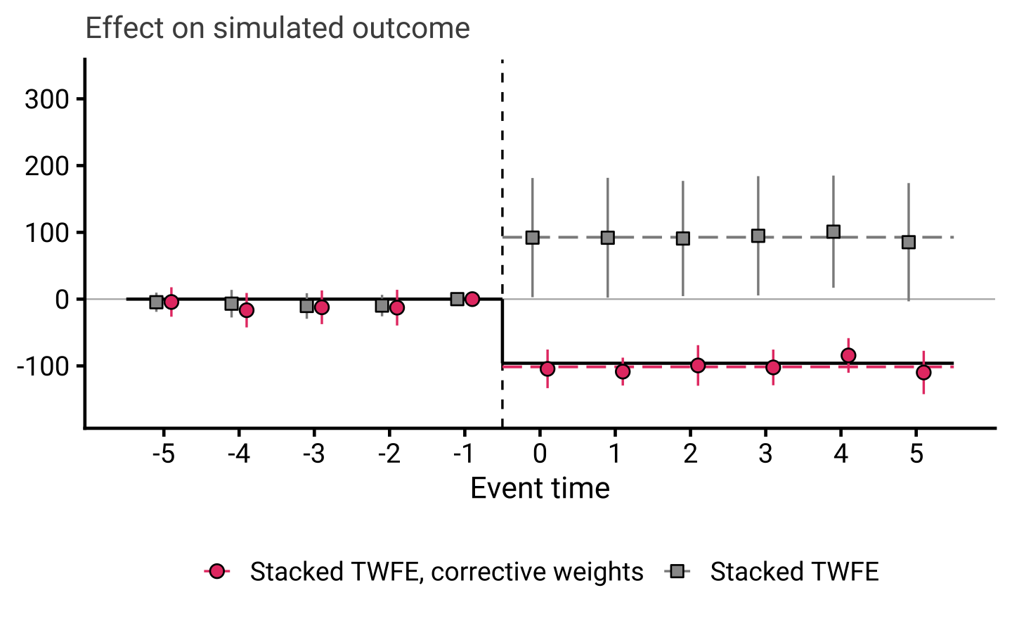
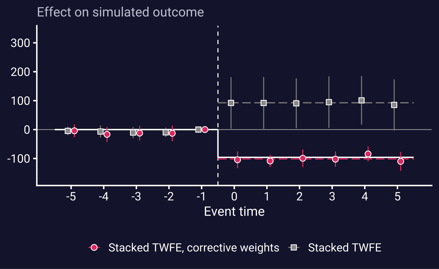
Here there are two treated cohorts who have treatment effects of opposite sign. Importantly, their sizes are wildly unequal. On this panel a stacked two-way-fixed-effects regression without corrective weights gets the sign of the average treatment effect wrong, while the corrective weights stacked TWFE estimator recovers the truth. Because there is noise, the numbers below are estimates with standard errors, not exact identities; they reproduce the paper’s Exhibit 2 and Table 1.
The deterministic signflip dataset that ships with the package is a noise-free miniature of this same scenario: 12 units across six years with worked numbers exactly reproduced. This is useful as a tool for seeing the mechanism without sampling variation. Below we use a noisy simulation.
The rest of this page rebuilds the sign-flip argument step by step, in three live figures: the raw group means, the sub-experiment weights that decide the sign, and the two event studies. A nice feature of this is that it walks through most of the functions in the package.
The data
The paper’s simulation ships as a helper on this site (assets/sim-signflip.R). It draws a 100-year panel for three groups: ten units that adopt in year 11 with a true effect of +300, a thousand units that adopt in year 60 with a true effect of −100, and ten never-treated units. Group, unit, and year fixed effects plus idiosyncratic noise are added in here, so recovered estimates may not perfectly reflect the true treatment effect for any given simulation run.
The large negative cohort dominates the treated mass, so the true average is negative, a fact the naive estimator will miss.
Raw trends by group
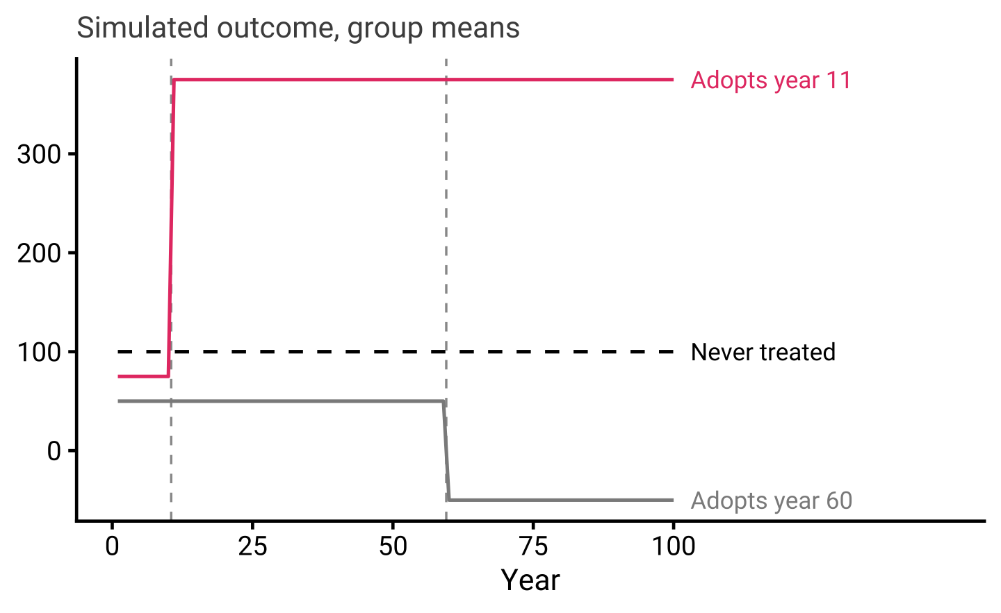
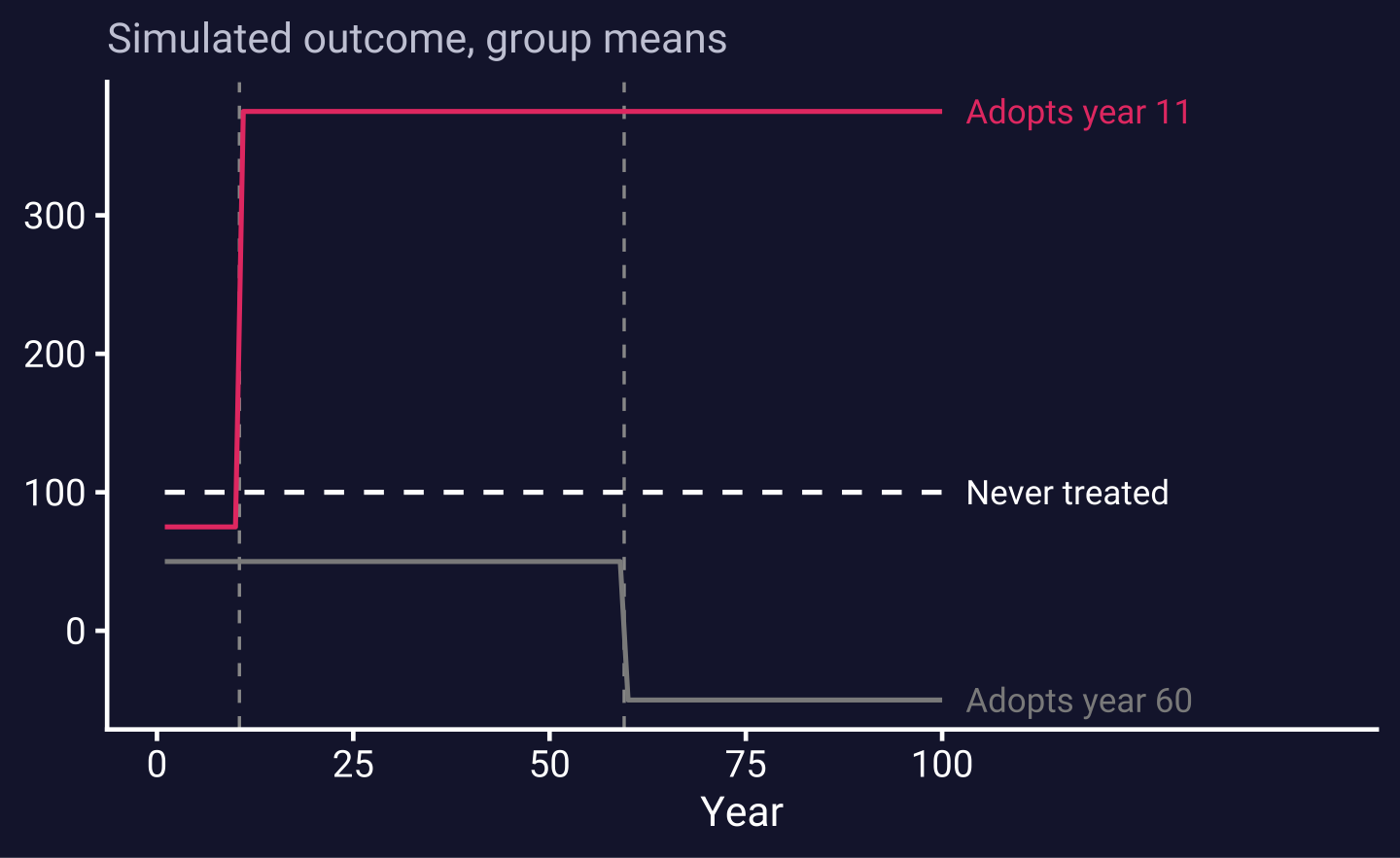
The mechanism is visible in the group means. The small year-11 cohort leaps up by 300 at adoption; the large year-60 cohort drops by 100 late in the panel; the never-treated units stay flat. (This raw panel is drawn from the noise-free group means, so the design reads cleanly; the event study and the weight scatter below use the full with-error series.)
Both cohorts have plenty of room inside a five-period window, so use \(\kappa_{\text{pre}} = \kappa_{\text{post}} = 5\) and draw controls from both the never-treated and the not-yet-treated units.
dd <- sim[, .(group_unit, year, adopt_year = time_treated, dep_var)]stack <-build_stack(dd, "year", "group_unit", "adopt_year",kappa_pre = KP, kappa_post = KQ,control_type ="both", weight_type ="unit_weights")# Q-weights: treated obs are 1. The large year-60 cohort has 1,000 treated# units but shares only a handful of controls, so its controls are upweighted# ~101x; the small year-11 cohort is swamped by controls, so its are pushed to 0.01.stack[, .(mean_q_weight =round(mean(q_weight), 2)), by = .(treat, sub_exp)][order(treat, sub_exp)]
stacked build, time(year) unit(group_unit) adopt(adopt_year) /// kpre(5) kpost(5) controltype(both) weighttype(unit_weights)* Q-weights by treatment status and cohorttable treat sub_exp, statistic(mean q_weight)
Naive versus Q-weighted
stackreg() applies the Q-weights automatically and returns the target. Running a plain, unweighted stacked TWFE on the same stack — treatment interacted with event time, absorbing unit-by-cohort and time-by-cohort fixed effects — gives the naive estimate.
The Q-weighted estimate is about −101 (SE 12.1) — right on the target of −96, within sampling noise. The naive stacked TWFE is about +93 (SE 44.5): not just biased, but the wrong sign. It overweights the small year-11 cohort, whose sub-experiment carries a disproportionate share of the treatment variance even though it holds barely 1% of the treated units.
Which weights, which sign
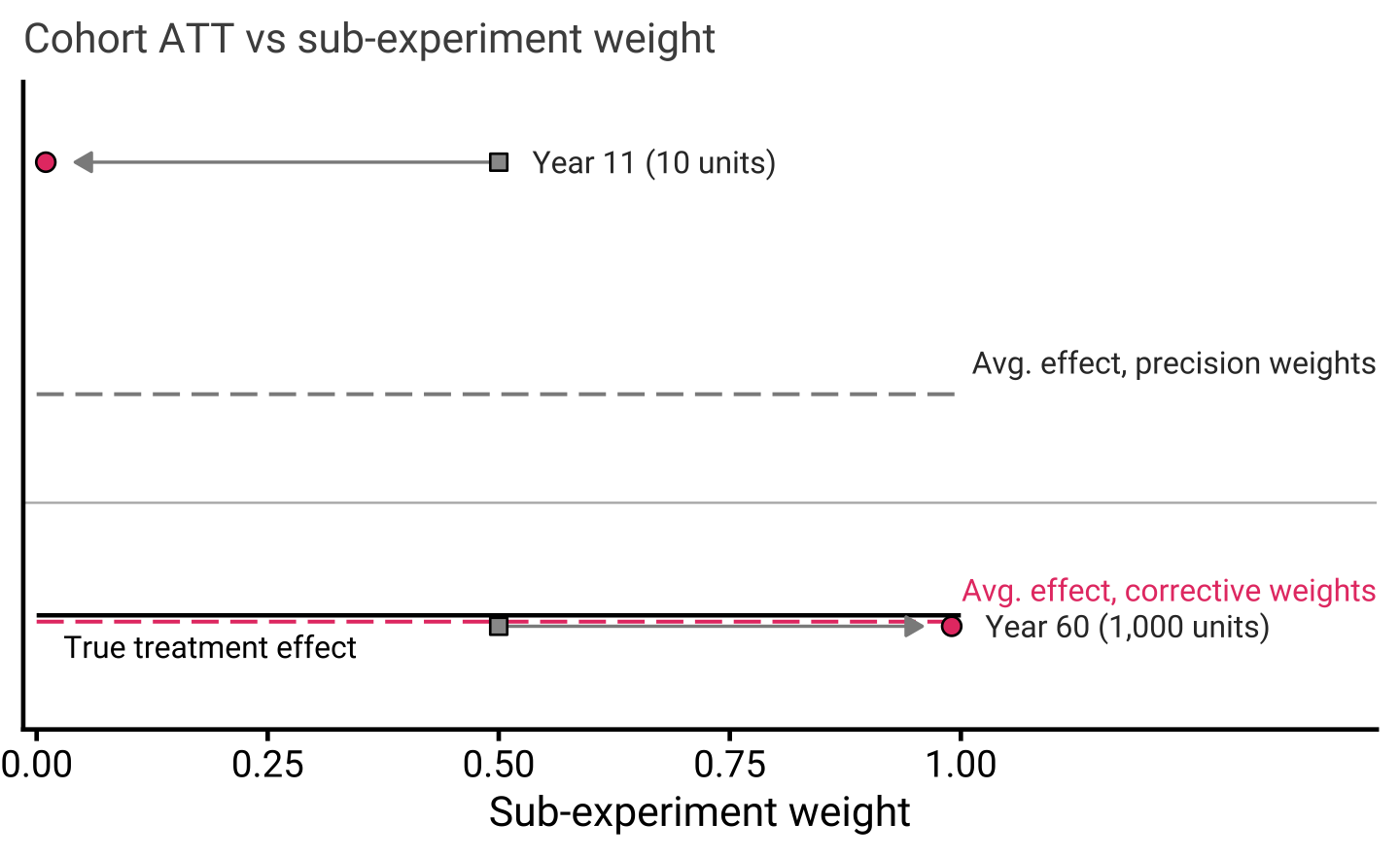
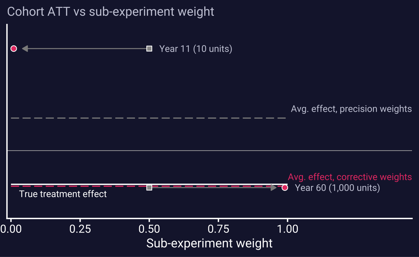
The choice of weights is the sign. Figure (b) plots each cohort’s own ATT against the weight its sub-experiment carries under the two schemes. Precision weighting (grey squares) splits the mass roughly 0.50/0.50 between the tiny +291 year-11 cohort and the huge −105 year-60 cohort, so its average lands above zero. Corrective weighting (pink circles) puts 0.99 on the large negative cohort — in proportion to its share of the treated units — and its average lands on the truth. The arrows show corrective weighting moving the mass from the precision to the treated-share allocation.
# Figure (b): each cohort's ATT against its sub-experiment weight (with error)p_mech <-sf_panel_mech(fx)
* stacked plot, bygroup overlays each cohort's ATT with marker size = weightstacked reg dep_var, cluster(group_unit) bygroupstacked plot, bygroup
Event study: only the corrective weights track the truth
Finally, the full event studies (figure c), with confidence intervals. The Q-weighted series (pink) is flat before adoption and settles near the truth of −96; the unweighted series (grey) sits on the wrong side of zero throughout the post-period.
Building a clean stack removed the negative-weights problem, but the unweighted regression on that clean stack still landed on the wrong side of zero. The Q-weights are what turn a clean design into a correct estimate. See stacking, aggregation issues, and corrective weights for the general argument and diagnostic divergence statistic, for the design diagnostic that flags this risk in advance.