library(stacked)
library(data.table)

# Load example data
data(medicaid)
head(medicaid)
#>    state statefip year adopt_year uninsured
#> 1:    AL        1 2008         NA 0.1964095
#> 2:    AL        1 2009         NA 0.2141095
#> 3:    AL        1 2010         NA 0.2300015
#> 4:    AL        1 2011         NA 0.2250678
#> 5:    AL        1 2012         NA 0.2159348
#> 6: AL 1 2013 NA 0.2218695Propensity Score Weighting for Stacked DID
Combining inverse-propensity weights with corrective Q-weights to target the ATT under covariate imbalance — in R and Stata.
Overview
This vignette explains when and how to incorporate propensity score weighting into stacked difference-in-differences analysis. The add_pscore_weights() function implements the methodology described in Appendix A4 of the Stacked DID working paper.
When to Use Propensity Score Weights
Standard Q-weights (computed by build_stack()) ensure proper aggregation across sub-experiments but do not address potential selection bias when treated and control units differ systematically on observed covariates.
Consider using propensity score weights when:
- Covariate imbalance exists: Treated and control groups differ on pre-treatment characteristics
- You want to improve robustness: Doubly-robust estimation combines outcome modeling with propensity score weighting
- You’re targeting the ATT: The inverse propensity weights implemented here target the average treatment effect on the treated
When propensity score weighting may not be necessary:
- The parallel trends assumption is well-supported by pre-trends
- Treated and control groups are well-balanced on observables
- You’re already including covariates in the outcome model
The Workflow
The propensity score weighting workflow has five steps:
- Build the stacked dataset with
build_stack() - Estimate propensity scores externally
- Add propensity scores to the stacked data
- Trim extreme propensity scores (user’s choice of bounds/strategy)
- Call
add_pscore_weights()to create adjusted Q-weights
* Load the bundled medicaid dataset
stacked use medicaid, clear
list in 1/6
Step 1: Build the Stacked Dataset
Start by building the stacked dataset as usual:
stack <- build_stack(
  data = medicaid,
  time_var = "year",
  unit_var = "state",
  adopt_var = "adopt_year",
  kappa_pre = 2,
  kappa_post = 2
)

# View structure
head(stack)
#>    state statefip year adopt_year uninsured sub_exp event_time treat post
#> 1:    AL        1 2012         NA 0.2159348    2014         -2     0    0
#> 2:    AL        1 2013         NA 0.2218695    2014         -1     0    0
#> 3:    AL        1 2014         NA 0.1980981    2014          0     0    1
#> 4:    AL        1 2015         NA 0.1741128    2014          1     0    1
#> 5:    AL        1 2016         NA 0.1574654    2014          2     0    1
#> 6:    AZ        4 2012       2014 0.2527074    2014         -2     1    0
#>    q_weight
#> 1: 2.888889
#> 2: 2.888889
#> 3: 2.888889
#> 4: 2.888889
#> 5: 2.888889
#> 6: 1.000000
* Build the stacked dataset (kpre=2, kpost=2)
stacked build, time(year) unit(state) adopt(adopt_year) ///
kpre(2) kpost(2)
list in 1/6Step 2: Estimate Propensity Scores
You estimate propensity scores externally, giving you full flexibility over the modeling approach. The propensity score should estimate the probability of being treated (in a given sub-experiment) conditional on covariates.
Simple Pooled Model
The simplest approach pools all observations:
# Example with a covariate (not available in medicaid data)
fit <- glm(treat ~ covariate1 + covariate2, family = binomial, data = stack)
stack[, phat := predict(fit, type = "response")]
Cell-by-Cell Estimation
For more flexibility, estimate separate models within each sub-experiment × event-time cell:
stack[, phat := {
  if (length(unique(treat)) == 2) {
    fit <- glm(treat ~ covariate1 + covariate2, family = binomial, data = .SD)
    predict(fit, type = "response")
  } else {
    # If all treated or all control in this cell, use overall mean
    mean(treat)
  }
}, by = .(sub_exp, event_time)]
Using Machine Learning
You can also use more sophisticated methods:
# Example with LASSO (requires glmnet)
library(glmnet)

X <- model.matrix(~ covariate1 + covariate2 + covariate3 - 1, data = stack)
cv_fit <- cv.glmnet(X, stack$treat, family = "binomial", alpha = 1)
stack[, phat := predict(cv_fit, newx = X, s = "lambda.min", type = "response")]
Demonstration with Simulated Covariate
For this demonstration, we’ll create a simulated covariate:
set.seed(123)

# Add a simulated covariate that's correlated with treatment status
# In practice, you would use actual covariates from your data
stack[, x_sim := rnorm(.N)]

# States that adopted treatment get slightly different x values
stack[treat == 1, x_sim := x_sim + 0.5]

# Estimate propensity scores
fit <- glm(treat ~ x_sim, family = binomial, data = stack)
stack[, phat := predict(fit, type = "response")]

# Check the distribution
summary(stack$phat)
#>    Min. 1st Qu.  Median    Mean 3rd Qu.    Max.
#> 0.09119 0.25615 0.33461 0.35000 0.42926 0.74477
Step 3: Trim Extreme Propensity Scores (If Needed)
Before adding propensity score weights, ensure all values are strictly between 0 and 1. Apply your preferred trimming strategy:
# Option 1: Drop observations with extreme propensity scores
# stack <- stack[phat > 0.01 & phat < 0.99]

# Option 2: Bound propensity scores (winsorize)
# This preserves sample size while limiting extreme weights
stack[, phat := pmin(pmax(phat, 0.01), 0.99)]

# Verify no extreme values remain
summary(stack$phat)
#>    Min. 1st Qu.  Median    Mean 3rd Qu.    Max.
#> 0.09119 0.25615 0.33461 0.35000 0.42926 0.74477
Step 4: Add Propensity Score Weights
Now use add_pscore_weights() to create adjusted Q-weights:
stack <- add_pscore_weights(
  stack_data = stack,
  pscore_var = "phat"
)

# New column q_weight_ps contains the adjusted weights
head(stack[, .(state, year, sub_exp, treat, q_weight, q_weight_ps)])
#>    state year sub_exp treat q_weight q_weight_ps
#> 1:    AL 2012    2014     0 2.888889    1.021725
#> 2:    AL 2013    2014     0 2.888889    1.234501
#> 3:    AL 2014    2014     0 2.888889    3.439165
#> 4:    AL 2015    2014     0 2.888889    1.466503
#> 5:    AL 2016    2014     0 2.888889    1.516714
#> 6:    AZ 2012    2014     1 1.000000    1.000000
* Create adjusted Q-weights from the propensity scores in phat
* (phat must already be in the data, strictly inside (0, 1))
stacked pscore, pscore(phat)
* New variable q_weight_ps holds the adjusted weights
list state year sub_exp treat q_weight q_weight_ps in 1/6The function:
- Computes inverse propensity weights (IPW): treated get weight 1, controls get weight p/(1-p)
- Uses these IPW weights to compute effective sample sizes
- Applies the Q-weight formula using the IPW-weighted counts
- Returns the final combined weight in
q_weight_ps
Step 5: Use in Regression
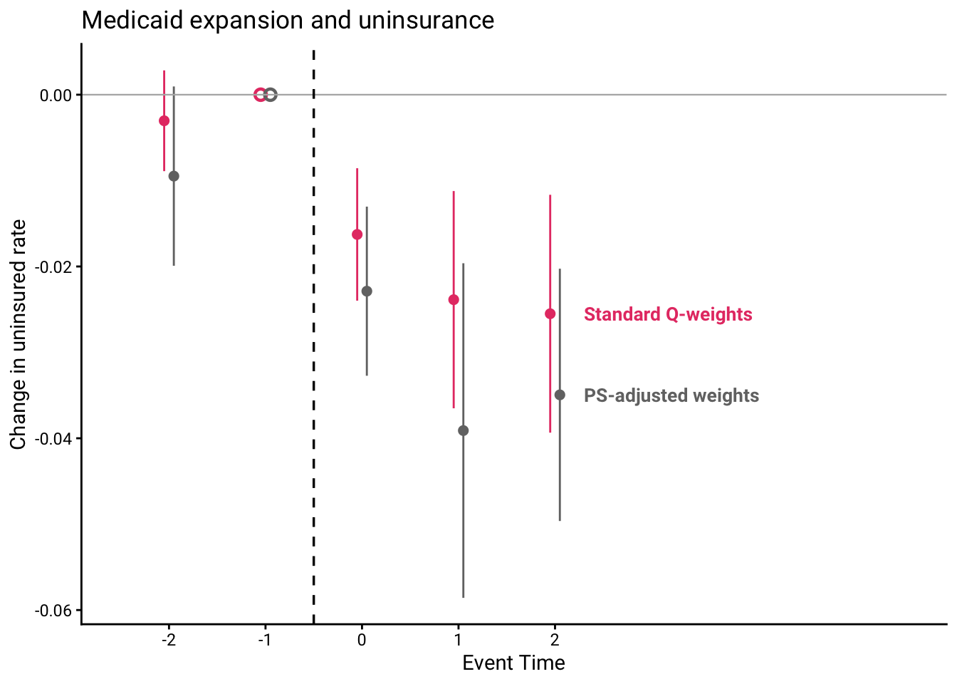
Fit the standard Q-weighted stack with stackreg(). For the propensity-adjusted weights we call fixest::feols() directly, because the custom q_weight_ps column is not the default q_weight that stackreg() uses. Both models have the standard treat:i(event_time) structure, so the package’s stack_coefs() and stack_plot_compare() read them directly.
library(fixest)

# Original regression with standard Q-weights
model_standard <- stackreg(stack, "uninsured", cluster_var = "state")

# Regression with propensity-score-adjusted weights
model_ps <- feols(
  uninsured ~ treat * i(event_time, ref = -1),
  data = stack,
  weights = ~q_weight_ps,
  cluster = ~state
)

# Compare event study coefficients as a house-style table
cs <- stack_coefs(model_standard)[, .(event_time, `Standard Q` = round(estimate, 4))]
cp <- stack_coefs(model_ps)[, .(event_time, `PS-adjusted` = round(estimate, 4))]
knitr::kable(
  merge(x = cs, y = cp, by = "event_time"),
  caption = "Event study coefficients: standard vs propensity-adjusted Q-weights"
)| event_time | Standard Q | PS-adjusted |
|---|---|---|
| -2 | -0.0030 | -0.0095 |
| -1 | 0.0000 | 0.0000 |
| 0 | -0.0163 | -0.0229 |
| 1 | -0.0239 | -0.0391 |
| 2 | -0.0255 | -0.0349 |
stack_plot_compare() overlays the two weightings in one event study, with the standard Q-weighted series in the highlight color and the propensity-adjusted series in grey:
stack_plot_compare(
  list(`Standard Q-weights` = model_standard,
       `PS-adjusted weights` = model_ps),
  title = "Medicaid expansion and uninsurance",
  ylab = "Change in uninsured rate"
)
* Standard Q-weighted event study
stacked reg uninsured, cluster(state) ref(-1)
stacked plot, title("Standard Q-weights")

* Propensity-score-adjusted Q-weights, then the event study
stacked pscore, pscore(phat)
stacked reg uninsured, cluster(state) ref(-1)
stacked plot, title("PS-adjusted weights")
Understanding the Weights
The IPW Component
The inverse propensity weights for ATT are:
- Treated units: \(w_{ATT} = 1\)
- Control units: \(w_{ATT} = \frac{p}{1-p}\)
where \(p\) is the propensity score. This upweights control units that are similar to treated units (high propensity score) and downweights those that are dissimilar.
The Q-Weight Component
The standard Q-weight formula adjusts for differential sub-experiment composition. With propensity score weighting, we compute Q-weights using the IPW-weighted counts instead of raw counts.
The Final Weight
The final weight combines both components:
\[w_{final} = w_{ATT} \times Q^{w_{ATT}}\]
Handling Extreme Propensity Scores
Extreme propensity scores (near 0 or 1) can lead to highly variable weights and unstable estimates. The add_pscore_weights() function requires propensity scores to be strictly between 0 and 1, and will error if any values are at the boundaries.
Recommended workflow: Apply your own trimming rules before calling the function. This gives you full control over the trimming strategy:
# Check the distribution of propensity scores
summary(stack$phat)
#>    Min. 1st Qu.  Median    Mean 3rd Qu.    Max.
#> 0.09119 0.25615 0.33461 0.35000 0.42926 0.74477

# Apply trimming to remove extreme values
# Choose bounds appropriate for your application
stack_trimmed <- stack[phat > 0.01 & phat < 0.99]

cat("Rows before trimming:", nrow(stack), "\n")
#> Rows before trimming: 500
cat("Rows after trimming:", nrow(stack_trimmed), "\n")
#> Rows after trimming: 500

# Now add propensity score weights
# Q-weights are recomputed from the trimmed data
stack_trimmed <- add_pscore_weights(
  stack_trimmed,
  pscore_var = "phat"
)
Why user-applied trimming? This approach:
- Gives you control over trimming bounds (0.01/0.99, 0.05/0.95, etc.)
- Allows alternative trimming strategies (winsorizing, dropping only one tail)
- Ensures Q-weights are correctly recomputed for the trimmed sample
Working with Survey Weights (Micro Data)
If you have micro data with survey weights, include them via weight_var:
# Example with survey weights
stack_micro <- add_pscore_weights(
  stack_data = stack_micro,
  pscore_var = "phat",
  weight_var = "survey_weight"
)
* Combine survey weights with the propensity-score adjustment
stacked pscore, pscore(phat) weightvar(survey_weight) datatype(rcs)The function will:
- Combine survey weights with IPW weights
- Use combined weights for computing effective sample sizes
- Apply the Q-weight formula appropriate for repeated cross-sections
Checking Balance
After applying propensity score weights, check whether covariate balance improved:
# Unweighted means
unweighted_balance <- stack[, .(
  mean_x_treated = mean(x_sim[treat == 1]),
  mean_x_control = mean(x_sim[treat == 0])
)]

# Weighted means (using propensity-adjusted weights)
weighted_balance <- stack[, .(
  mean_x_treated = weighted.mean(x_sim[treat == 1], q_weight_ps[treat == 1]),
  mean_x_control = weighted.mean(x_sim[treat == 0], q_weight_ps[treat == 0])
)]

# Compare
cat("Unweighted:\n")
#> Unweighted:
print(unweighted_balance)
#>    mean_x_treated mean_x_control
#> 1:      0.5626693     0.01947108

cat("\nWeighted:\n")
#>
#> Weighted:
print(weighted_balance)
#>    mean_x_treated mean_x_control
#> 1:      0.5626693      0.5653874

cat("\nDifference reduced:",
    abs(unweighted_balance$mean_x_treated - unweighted_balance$mean_x_control) >
    abs(weighted_balance$mean_x_treated - weighted_balance$mean_x_control))
#>
#> Difference reduced: TRUE
Best Practices
Estimate propensity scores carefully: The quality of propensity score weighting depends on correct model specification
Check overlap: Ensure there are both treated and control units at all propensity score levels. The function checks for this at the cell level.
Examine weight distribution: Very large or small weights may indicate poor overlap or model misspecification
Compare results: If propensity-score-weighted results differ substantially from standard results, investigate why
Consider doubly-robust estimation: Combine propensity score weighting with covariate adjustment in the outcome model for extra robustness
Summary
The add_pscore_weights() function provides a straightforward way to incorporate propensity score weighting into stacked DID analysis. The key workflow is:
build_stack()- Create the stacked dataset- Estimate propensity scores externally
- Trim extreme propensity scores (your choice of bounds)
add_pscore_weights()- Create adjusted Q-weights- Use
q_weight_psin your regression
This approach maintains the benefits of the stacked DID method while addressing potential covariate imbalance between treated and control groups. The user-applied trimming step ensures you have full control over the trimming strategy, and the Q-weights are correctly recomputed for the (possibly trimmed) sample.
References
Wing, C., Hollingsworth, A., & Freedman, S. (2024). Stacked Difference-in-Differences. Working Paper. Appendix A4.