library(stacked)
library(data.table)

# Load the example dataset
data(medicaid)
head(medicaid)
#>    state statefip year adopt_year uninsured
#> 1:    AL        1 2008         NA 0.1964095
#> 2:    AL        1 2009         NA 0.2141095
#> 3:    AL        1 2010         NA 0.2300015
#> 4:    AL        1 2011         NA 0.2250678
#> 5:    AL        1 2012         NA 0.2159348
#> 6: AL 1 2013 NA 0.2218695Introduction to Stacked Difference-in-Differences
The core stacked DID workflow — explore kappas, build the stack, estimate, and visualize — in R and Stata.
Overview
The stacked package implements the stacked difference-in-differences (DID) method for causal inference with staggered treatment adoption. This approach is particularly useful when:
- Different units adopt treatment at different times
- You want to avoid the biases that can arise with two-way fixed effects (TWFE)
- You want transparent, interpretable event study estimates
This vignette walks through the core workflow using the included medicaid dataset, which contains state-level uninsurance rates and ACA Medicaid expansion adoption dates.
The Problem with Staggered Adoption
When treatment is adopted at different times across units, standard TWFE regressions can produce biased estimates. This happens because TWFE implicitly uses already-treated units as controls for later-treated units, which can lead to negative weights and misleading conclusions.
The stacked DID approach solves this by:
- Creating separate “sub-experiments” for each adoption cohort
- Using only clean controls (never-treated or not-yet-treated units)
- Aligning observations by event time rather than calendar time
- Applying corrective weights to ensure proper aggregation
Getting Started
* Load the bundled medicaid dataset
stacked use medicaid, clear
list in 1/6
The medicaid dataset contains:
state: Two-letter state abbreviationstatefip: State FIPS codeyear: Calendar year (2008-2021)adopt_year: Year of Medicaid expansion adoption (NA if not adopted)uninsured: Fraction of adults ages 18-60 without health insurance
Step 1: Explore Kappa Trade-offs
Before building the stacked dataset, it’s helpful to understand how different choices of kappa_pre (pre-treatment periods) and kappa_post (post-treatment periods) affect your analysis.
# Explore different kappa combinations
tradeoffs <- kappa_trade_offs(
  data = medicaid,
  time_var = "year",
  unit_var = "state",
  adopt_var = "adopt_year",
  kappa_pre_range = 1:4,
  kappa_post_range = 1:4
)

# View a subset of the results
tradeoffs[kappa_pre <= 3 & kappa_post <= 3]
#>    kappa_pre kappa_post n_sub_exp n_unidentified_sub_exp n_event_times n_obs
#> 1:         1          1         5                      0             3   354
#> 2:         1          2         4                      0             4   400
#> 3:         1          3         3                      0             5   425
#> 4:         2          1         5                      0             4   472
#> 5:         2          2         4                      0             5   500
#> 6:         2          3         3                      0             6   510
#> 7:         3          1         5                      0             5   590
#> 8:         3          2         4                      0             6   600
#> 9:         3          3         3                      0             7   595
#>    total_treated_obs total_control_obs avg_treated_per_period
#> 1:               114               240                     38
#> 2:               140               260                     35
#> 3:               165               260                     33
#> 4:               152               320                     38
#> 5:               175               325                     35
#> 6:               198               312                     33
#> 7:               190               400                     38
#> 8:               210               390                     35
#> 9:               231               364                     33
#>    avg_control_per_period sd_treated_per_period sd_control_per_period
#> 1:                     80                     0                     0
#> 2:                     65                     0                     0
#> 3:                     52                     0                     0
#> 4:                     80                     0                     0
#> 5:                     65                     0                     0
#> 6:                     52                     0                     0
#> 7:                     80                     0                     0
#> 8:                     65                     0                     0
#> 9:                     52                     0                     0
#>              adoption_times_str
#> 1: 2014, 2015, 2016, 2019, 2020
#> 2:       2014, 2015, 2016, 2019
#> 3:             2014, 2015, 2016
#> 4: 2014, 2015, 2016, 2019, 2020
#> 5:       2014, 2015, 2016, 2019
#> 6:             2014, 2015, 2016
#> 7: 2014, 2015, 2016, 2019, 2020
#> 8:       2014, 2015, 2016, 2019
#> 9:             2014, 2015, 2016
* Explore different kappa combinations (grid over kpre and kpost)
stacked kappa, time(year) unit(state) adopt(adopt_year) ///
kpre(1/4) kpost(1/4)
* The full grid is returned in r(table)
matrix list r(table)Key columns in the output:
- n_sub_exp: Number of adoption cohorts (sub-experiments) included
- n_event_times: Number of event-time periods (kappa_pre + kappa_post + 1)
- n_obs: Total observations in the stacked dataset
- total_treated_obs / total_control_obs: Total treated and control observations
- avg_treated_per_period / avg_control_per_period: Average counts per event-time
- adoption_times_str: Which adoption cohorts are included
These statistics match exactly what build_stack() produces. You can verify: n_obs = total_treated_obs + total_control_obs.
Larger kappa values give you longer event windows but exclude cohorts near the data boundaries. Choose values that balance your research needs.
Step 2: Build the Stacked Dataset
Once you’ve chosen your kappa values, use build_stack() to create the stacked dataset:
# Build stacked dataset with kappa_pre=3, kappa_post=2
stack <- build_stack(
  data = medicaid,
  time_var = "year",
  unit_var = "state",
  adopt_var = "adopt_year",
  kappa_pre = 3,
  kappa_post = 2
)

# View structure
str(stack)
#> Classes 'data.table' and 'data.frame':   600 obs. of  10 variables:
#>  $ state     : chr  "AL" "AL" "AL" "AL" ...
#>  $ statefip  : int  1 1 1 1 1 1 4 4 4 4 ...
#>  $ year      : int  2011 2012 2013 2014 2015 2016 2011 2012 2013 2014 ...
#>  $ adopt_year: int  NA NA NA NA NA NA 2014 2014 2014 2014 ...
#>  $ uninsured : num  0.225 0.216 0.222 0.198 0.174 ...
#>  $ sub_exp   : int  2014 2014 2014 2014 2014 2014 2014 2014 2014 2014 ...
#>  $ event_time: int  -3 -2 -1 0 1 2 -3 -2 -1 0 ...
#>  $ treat     : int  0 0 0 0 0 0 1 1 1 1 ...
#>  $ post      : int  0 0 0 1 1 1 0 0 0 1 ...
#>  $ q_weight  : num  2.89 2.89 2.89 2.89 2.89 ...
#>  - attr(*, ".internal.selfref")=<externalptr>
#>  - attr(*, "index")= int(0)
#>   ..- attr(*, "__treat")= int [1:600] 1 2 3 4 5 6 49 50 51 52 ...
#>  - attr(*, "stacked_meta")=List of 9
#>   ..$ weight_type: chr "unit_weights"
#>   ..$ pop_var    : NULL
#>   ..$ weight_var : NULL
#>   ..$ unit_var   : chr "state"
#>   ..$ time_var   : chr "year"
#>   ..$ adopt_var  : chr "adopt_year"
#>   ..$ data_type  : chr "panel"
#>   ..$ kappa_pre  : num 3
#>   ..$ kappa_post : num 2

# Key new columns
head(stack[, .(state, year, adopt_year, sub_exp, event_time, treat, q_weight)])
#>    state year adopt_year sub_exp event_time treat q_weight
#> 1:    AL 2011         NA    2014         -3     0 2.888889
#> 2:    AL 2012         NA    2014         -2     0 2.888889
#> 3:    AL 2013         NA    2014         -1     0 2.888889
#> 4:    AL 2014         NA    2014          0     0 2.888889
#> 5:    AL 2015         NA    2014          1     0 2.888889
#> 6:    AL 2016         NA    2014          2     0 2.888889
* Build the stacked dataset in memory (replaces the data with the stack)
stacked build, time(year) unit(state) adopt(adopt_year) ///
kpre(3) kpost(2)
* Key new variables
list state year adopt_year sub_exp event_time treat q_weight in 1/6The function adds several columns:
- sub_exp: Sub-experiment identifier (equals the adoption year)
- event_time: Time relative to treatment (-3, -2, -1, 0, 1, 2)
- treat: Treatment indicator (1 for treated units in this sub-experiment)
- post: Post-treatment indicator
- q_weight: The corrective weight for proper aggregation
Understanding Q-Weights
The Target Aggregate Parameter
With staggered adoption, we identify separate group-time average treatment effects (ATTs) for each adoption cohort at each event time. In practice, we usually want to combine these into a summary measure. But how should we combine them?
The stacked DID approach takes a forward-engineering perspective: we first define a target aggregate parameter that combines the underlying group-time ATTs in a sensible way. The default target is the trimmed aggregate ATT:
\[\theta_{\kappa}^{e} = \sum_{a \in \Omega_{\kappa}} ATT(a,a+e) \times \frac{N_{a}^{D}}{N_{\Omega_{\kappa}}^{D}}\]
This weights each group-time ATT by its share of the treated units in the trimmed set. For example, if one adoption cohort contains 60% of the treated units and another contains 40%, the aggregate weights their effects accordingly. The composition remains constant across event times, so changes in the aggregate over time reflect dynamics rather than composition.
Why Stacking Alone Isn’t Enough
Building a stacked dataset with compositionally balanced sub-experiments solves many problems with staggered adoption designs. In particular, it avoids using already-treated units as controls for later-treated units, which is the source of the “negative weights” problem with two-way fixed effects.
However, stacking alone does not guarantee that an ordinary least squares regression on the stacked data recovers the target aggregate parameter. The issue is subtle: when the ratio of treated to control units differs across sub-experiments, an unweighted regression implicitly averages treatment-group trends and control-group trends using different weights. Even if the parallel trends assumption holds within each sub-experiment, these differential weights can cause bias.
How Q-Weights Correct for This
The Q-weights correct for sample size imbalances across sub-experiments so that the weighted least squares regression targets the parameter we set out to estimate. For treated observations, the Q-weight is simply 1. For control observations in sub-experiment \(a\), the weight is:
\[Q_{a} = \frac{N_a^D / N_{\Omega}^D}{N_a^C / N_{\Omega}^C}\]
This rescales each control observation so that, effectively, the same weighting scheme is applied to both treatment and control group trends. The differential weighting problem cancels out, and the regression coefficients identify the target aggregate.
# Q-weights for treated units are always 1
stack[treat == 1, summary(q_weight)]
#>    Min. 1st Qu.  Median    Mean 3rd Qu.    Max.
#>       1       1       1       1       1       1

# Q-weights for control units vary by sub-experiment composition
stack[treat == 0, .(mean_weight = mean(q_weight)), by = sub_exp]
#>    sub_exp mean_weight
#> 1:    2014   2.8888889
#> 2:    2015   0.3095238
#> 3:    2016   0.2063492
#> 4:    2019   0.3376623
Different Weights for Different Targets
The weight_type parameter in build_stack() lets you target different aggregate parameters:
"unit_weights"(default): Each group-time ATT is weighted by its share of treated units. Adoption cohorts with more treated units contribute more."population_between": Each group-time ATT is weighted by its share of the treated population (requires a population variable). Useful when units represent geographic areas of different sizes."pop_constant": Full population weighting (between AND within sub-experiments) for constant populations. Weights effects by people rather than administrative units."pop_total_periods": Full population weighting for time-varying populations. Uses total population-periods as the within-sub-experiment weight, producing time-invariant Q-weights."pop_period_specific": Full population weighting for time-varying populations. Uses period-specific population directly, so Q-weights vary across event times."sample_share": Each group-time ATT is weighted by its share of the full stacked sample (treated + control). Sub-experiments with larger overall samples contribute more.
All of these are valid aggregation schemes that define different estimands. Which is appropriate depends on the research question.
Practical Considerations
In many applications, the Q-weights make only modest differences to the point estimates. This happens when the treated-to-control ratio is similar across sub-experiments, or when group-time ATTs don’t vary much. Still, using the Q-weights is the principled approach because it ensures your estimates correspond to a well-defined target parameter—and the weights can matter substantially when sub-experiments differ in composition.
Step 3: Fit the Event Study Regression
With the stacked dataset ready, you can fit the weighted event study regression:
# Fit the regression (requires fixest package)
model <- stackreg(
  stack_data = stack,
  outcome_var = "uninsured",
  cluster_var = "state",
  ref_period = -1  # Reference period (immediately before treatment)
)

# View results
summary(model)
#> OLS estimation, Dep. Var.: uninsured
#> Observations: 600
#> Weights: stack_data$q_weight
#> Standard-errors: Clustered (state)
#>                       Estimate Std. Error    t value   Pr(>|t|)
#> (Intercept)           0.215541   0.010271  20.985134  < 2.2e-16 ***
#> treat                -0.041182   0.013442  -3.063708 3.5171e-03 **
#> event_time::-3        0.011275   0.002031   5.552085 1.0776e-06 ***
#> event_time::-2        0.007027   0.002221   3.163728 2.6496e-03 **
#> event_time::0        -0.025362   0.001840 -13.780979  < 2.2e-16 ***
#> event_time::1        -0.044675   0.003355 -13.315708  < 2.2e-16 ***
#> event_time::2        -0.052770   0.003836 -13.757047  < 2.2e-16 ***
#> treat:event_time::-3 -0.001022   0.003683  -0.277565 7.8249e-01
#> treat:event_time::-2 -0.003035   0.002993  -1.013768 3.1557e-01
#> treat:event_time::0  -0.016270   0.003934  -4.135735 1.3516e-04 ***
#> treat:event_time::1  -0.023864   0.006454  -3.697642 5.4101e-04 ***
#> treat:event_time::2  -0.025500   0.007066  -3.608715 7.1081e-04 ***
#> ---
#> Signif. codes:  0 '***' 0.001 '**' 0.01 '*' 0.05 '.' 0.1 ' ' 1
#> RMSE: 0.04462   Adj. R2: 0.417048
* Fit the Q-weighted event-study regression (reference period -1)
stacked reg uninsured, cluster(state) ref(-1)The coefficients on the treat:event_time interactions are your event study estimates. They represent the effect of Medicaid expansion on uninsurance at each event time, relative to the period just before treatment.
Step 4: Visualize Results
Create an event study plot to visualize the treatment effects:
# Create the event study plot
p <- stack_plot(
  model,
  title = "Effect of Medicaid Expansion on Uninsurance",
  ylab = "Change in Uninsured Rate"
)
print(p)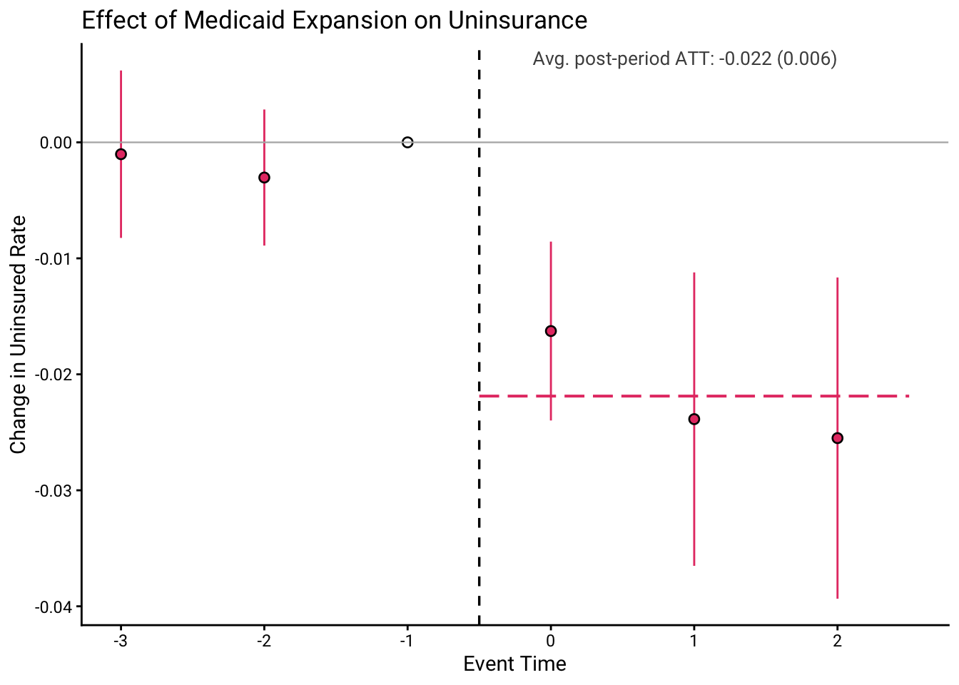
* Plot the event study coefficients from the last stacked reg
stacked plot, title("Effect of Medicaid Expansion on Uninsurance")
Interpreting the plot:
- Pre-treatment coefficients (event_time < 0) should be near zero if the parallel trends assumption holds
- Post-treatment coefficients (event_time >= 0) show the dynamic treatment effects
- The vertical dashed line marks the treatment date
Step 5: Visualize Outcome Levels
The event study coefficients show treatment effects relative to the reference period. Sometimes it is also useful to plot the Q-weighted mean of the outcome itself for treatment and control groups over the event window. This shows the raw level of the outcome, which can help readers understand the magnitude of the effect in context.
# Plot Q-weighted mean outcome levels
p_levels <- stack_plot_levels(
  stack, "uninsured",
  ylab = "Uninsured Rate"
)
print(p_levels)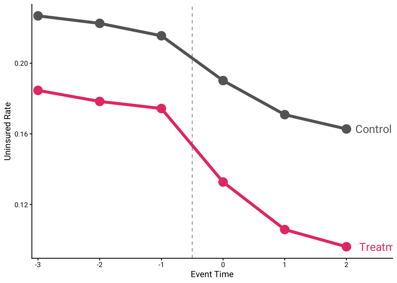
* Plot the Q-weighted mean outcome levels for treated and control groups
stacked levels uninsured, plot
The function uses the Q-weights from build_stack() when computing means, so the treatment and control averages reflect the same target estimand as the regression. If you built your stack with different weight_type options (e.g., population weights), the level plot will reflect that weighting.
You can also extract the underlying means as a data.table using stack_levels():
levels_dt <- stack_levels(stack, "uninsured")
print(levels_dt)
#>    event_time treat_mean_uninsured control_mean_uninsured
#> 1:         -3           0.18461237              0.2268165
#> 2:         -2           0.17835218              0.2225687
#> 3:         -1           0.17435925              0.2155412
#> 4:          0           0.13272761              0.1901791
#> 5:          1           0.10582017              0.1708659
#> 6:          2           0.09608882              0.1627709
* Extract the Q-weighted means (returned in r(levels))
stacked levels uninsured
matrix list r(levels)The column names include the outcome variable (e.g., treat_mean_uninsured, control_mean_uninsured), so you can merge results from multiple outcomes without column name conflicts:
# Merge level means from two outcomes
levels1 <- stack_levels(stack, "outcome1")
levels2 <- stack_levels(stack, "outcome2")
merged <- merge(levels1, levels2, by = "event_time")
Using Your Own Regression
One advantage of stacked is that you can use the stacked data with any regression package. The key is to use the q_weight column as weights and to set the reference period to event_time = -1 (the period just before treatment).
Using base R lm()
# Create event_time factor with -1 as reference level
stack[, event_time_f := relevel(factor(event_time), ref = "-1")]

# Fit weighted regression
model_lm <- lm(
  uninsured ~ treat * event_time_f,
  data = stack,
  weights = q_weight
)

# Extract event study coefficients
coefs <- coef(model_lm)
event_coefs <- coefs[grep("treat:event_time_f", names(coefs))]
print(event_coefs)
#> treat:event_time_f-3 treat:event_time_f-2  treat:event_time_f0
#>         -0.001022172         -0.003034560         -0.016269503
#>  treat:event_time_f1  treat:event_time_f2
#>         -0.023863697         -0.025500057
Using fixest::feols()
The fixest package offers faster estimation and convenient syntax for event studies:
library(fixest)

# feols with i() automatically handles factor creation and reference period
model_feols <- feols(
  uninsured ~ treat * i(event_time, ref = -1),
  data = stack,
  weights = ~q_weight,
  cluster = ~state
)

# View coefficients
coeftable(model_feols)[grep("treat:event_time", rownames(coeftable(model_feols))), ]
#>                          Estimate  Std. Error    t value     Pr(>|t|)
#> treat:event_time::-3 -0.001022172 0.003682642 -0.2775648 0.7824909171
#> treat:event_time::-2 -0.003034560 0.002993349 -1.0137676 0.3155744181
#> treat:event_time::0  -0.016269503 0.003933884 -4.1357350 0.0001351557
#> treat:event_time::1  -0.023863697 0.006453761 -3.6976419 0.0005410142
#> treat:event_time::2  -0.025500057 0.007066243 -3.6087151 0.0007108064
Control Type Options
By default, build_stack() uses both never-treated and not-yet-treated units as controls. You can change this:
# Never-treated only
stack_never <- build_stack(
  medicaid, "year", "state", "adopt_year",
  kappa_pre = 3, kappa_post = 2,
  control_type = "never_treated"
)

# Not-yet-treated only
stack_notyet <- build_stack(
  medicaid, "year", "state", "adopt_year",
  kappa_pre = 3, kappa_post = 2,
  control_type = "not_yet_treated"
)
#> Warning: Dropped 1 unidentified sub-experiment(s) with no eligible control
#> units: 2019 (no unit adopts more than kappa_post = 2 periods after these
#> cohorts; consider control_type = 'both' or a smaller kappa_post). Their
#> event-time effects are not identified, and keeping them would assign Q-weight
#> mass to cohorts that contribute no information.

# Compare sample sizes
cat("Both controls:", nrow(stack), "obs\n")
#> Both controls: 600 obs
cat("Never-treated only:", nrow(stack_never), "obs\n")
#> Never-treated only: 474 obs
cat("Not-yet-treated only:", nrow(stack_notyet), "obs\n")
#> Not-yet-treated only: 324 obs
* Never-treated only
stacked use medicaid, clear
stacked build, time(year) unit(state) adopt(adopt_year) ///
kpre(3) kpost(2) controltype(never)
* Not-yet-treated only
stacked use medicaid, clear
stacked build, time(year) unit(state) adopt(adopt_year) ///
kpre(3) kpost(2) controltype(notyet)Restricting Not-Yet-Treated Controls with nyt_horizon
By default, any unit that adopts treatment after the sub-experiment observation window qualifies as a not-yet-treated control. The nyt_horizon parameter lets you restrict this pool to units adopting within a specified number of periods after the window.
For a sub-experiment with focal adoption time a and post-window kappa_post, setting nyt_horizon = m restricts not-yet-treated controls to those with adopt_var > a + kappa_post and adopt_var <= a + kappa_post + m.
# Only controls adopting within 3 periods after the window
stack_h3 <- build_stack(
  medicaid, "year", "state", "adopt_year",
  kappa_pre = 3, kappa_post = 2,
  control_type = "not_yet_treated",
  nyt_horizon = 3
)
#> Warning: Dropped 1 unidentified sub-experiment(s) with no eligible control
#> units: 2019 (no unit adopts more than kappa_post = 2 periods after these
#> cohorts; consider control_type = 'both' or a smaller kappa_post). Their
#> event-time effects are not identified, and keeping them would assign Q-weight
#> mass to cohorts that contribute no information.

# Compare: unrestricted vs. restricted not-yet-treated
cat("Unrestricted NYT:", nrow(stack_notyet), "obs\n")
#> Unrestricted NYT: 324 obs
cat("NYT horizon = 3:", nrow(stack_h3), "obs\n")
#> NYT horizon = 3: 282 obs

# nyt_horizon also works with control_type = "both"
stack_both_h3 <- build_stack(
  medicaid, "year", "state", "adopt_year",
  kappa_pre = 3, kappa_post = 2,
  control_type = "both",
  nyt_horizon = 3
)
cat("Both with horizon = 3:", nrow(stack_both_h3), "obs\n")
#> Both with horizon = 3: 558 obs
* Only controls adopting within 3 periods after the window
stacked use medicaid, clear
stacked build, time(year) unit(state) adopt(adopt_year) ///
kpre(3) kpost(2) controltype(notyet) nythorizon(3)
* nyt_horizon also works with controltype(both)
stacked use medicaid, clear
stacked build, time(year) unit(state) adopt(adopt_year) ///
kpre(3) kpost(2) controltype(both) nythorizon(3)Weight Type Options
The weight_type parameter controls what estimand the Q-weights target. There are six options:
"unit_weights"(default): Weights sub-experiments by the number of treated units, so cohorts with more treated units contribute more to the overall estimate."population_between": Weights sub-experiments by the population of treated units, but units within each sub-experiment receive equal weight. Requires specifyingpop_varwith a variable containing population counts."pop_constant": Full population weighting – weights both between sub-experiments (by treated population share) AND within sub-experiments (by unit population). Assumes constant population within units (Appendix 0, Constant Population Size case). Use this when the research question concerns effects on people rather than administrative units. Requirespop_var."pop_total_periods": Like"pop_constant"but for time-varying populations. Uses total population-periods (pe_sa = sum_e p_sae) within each sub-experiment as the within-sub-experiment weight. Q-weights are constant across event times for a given unit within a sub-experiment (Appendix 0, Time Varying Population Weights case). Requirespop_var."pop_period_specific": Like"pop_constant"but for time-varying populations. Uses the period-specific populationp_saedirectly as the within-sub-experiment weight. Unlike"pop_total_periods", Q-weights vary across event times, reflecting the actual population present in each period. Requirespop_var."sample_share": Equal-weighted across sub-experiments. Each adoption cohort contributes equally to the overall estimate, regardless of the number of treated units.
The deprecated names "att" and "pop_time_varying" are silently accepted as aliases for "unit_weights" and "pop_total_periods", respectively.
# Default unit weights (by treated unit counts)
stack_unit <- build_stack(
  medicaid, "year", "state", "adopt_year",
  kappa_pre = 3, kappa_post = 2,
  weight_type = "unit_weights"
)

# Sample share weights (equal weight per cohort)
stack_ss <- build_stack(
  medicaid, "year", "state", "adopt_year",
  kappa_pre = 3, kappa_post = 2,
  weight_type = "sample_share"
)

# Compare Q-weights for controls across sub-experiments
stack_unit[treat == 0, .(unit_weight = mean(q_weight)), by = sub_exp]
#>    sub_exp unit_weight
#> 1:    2014   2.8888889
#> 2:    2015   0.3095238
#> 3:    2016   0.2063492
#> 4:    2019   0.3376623
stack_ss[treat == 0, .(ss_weight = mean(q_weight)), by = sub_exp]
#>    sub_exp ss_weight
#> 1:    2014 1.6611111
#> 2:    2015 0.7583333
#> 3:    2016 0.7222222
#> 4:    2019 0.7681818
* Default unit weights (by treated unit counts)
stacked use medicaid, clear
stacked build, time(year) unit(state) adopt(adopt_year) ///
kpre(3) kpost(2) weighttype(unit_weights)
* Sample share weights (equal weight per cohort)
stacked use medicaid, clear
stacked build, time(year) unit(state) adopt(adopt_year) ///
kpre(3) kpost(2) weighttype(sample_share)For population-weighted estimates (useful when states or units have very different sizes), you need to provide a population variable:
# Example with population weights (requires population variable)
stack_pop <- build_stack(
  data = state_data,
  time_var = "year",
  unit_var = "state",
  adopt_var = "adopt_year",
  kappa_pre = 3,
  kappa_post = 2,
  weight_type = "population_between",
  pop_var = "state_population"
)
* Example with population weights (requires a population variable)
stacked build, time(year) unit(state) adopt(adopt_year) ///
kpre(3) kpost(2) weighttype(population_between) popvar(state_population)When to use each weight type:
- Use
"unit_weights"(default) when you want each treated unit to contribute equally - Use
"population_between"when sub-experiments with larger treated populations should count more, but units within each sub-experiment receive equal weight - Use
"pop_constant"when you want full population weighting (between AND within sub-experiments) and population is constant within units - Use
"pop_total_periods"when you want full population weighting with time-varying populations and prefer time-invariant Q-weights within each unit-sub-experiment pair - Use
"pop_period_specific"when you want full population weighting with time-varying populations and want the weight to reflect the actual population present in each specific period - Use
"sample_share"when you want each adoption cohort to contribute equally, regardless of size
Working with Micro Data
For repeated cross-sectional data with survey weights (like individual-level ACS data), pass the weight variable to build_stack():
# Example with micro data (not run - requires micro dataset)
stack_micro <- build_stack(
  data = micro_data,
  time_var = "year",
  unit_var = "state",
  adopt_var = "adopt_year",
  kappa_pre = 3,
  kappa_post = 2,
  weight_var = "perwt"  # Survey weight variable
)
* Micro data with survey weights (repeated cross-sections)
stacked build, time(year) unit(state) adopt(adopt_year) ///
kpre(3) kpost(2) datatype(rcs) weightvar(perwt)When weight_var is specified, the Q-weights are computed using survey-weighted counts, and the final q_weight column is the product of the survey weight and the corrective weight.
Decomposing by timing group
Every pooled estimate above is a weighted average across adoption cohorts, with weights equal to each cohort’s share of treated Q-weight. Setting by_group = TRUE estimates the same model separately within each sub-experiment and returns the per-cohort estimates together with those weights, so you can see exactly which cohorts drive the pooled number:
groups <- stackreg(stack, "uninsured", cluster_var = "state",
                   by_group = TRUE)
groups
#> <stackreg_groups> event study by timing group (4 cohorts)
#>
#>    sub_exp        att         se    weight
#> 1:    2014 -0.0215517 0.00650243 0.8000000
#> 2:    2015 -0.0158562 0.00521068 0.0857143
#> 3:    2016 -0.0421334 0.00414854 0.0571429
#> 4:    2019 -0.0152191 0.00394367 0.0571429
#>
#> pooled: -0.0218778 (se 0.00562813);  weighted sum of cohort ATTs: -0.0218778
* Estimate the same model separately within each timing group
stacked reg uninsured, cluster(state) bygroup
* Per-cohort ATTs, weights, and the aggregation identity are in r(group_att)
matrix list r(group_att)The printed table reports each cohort’s ATT, its weight, and verifies the aggregation identity (pooled = sum of weight x cohort ATT). Pass the object to stack_plot() for an overlaid event study (point size = cohort weight, pooled estimate in black), or stack_plot(groups, combine = "facet") for one panel per cohort. If the cohorts were fit with stackreg(..., model = "att", by_group = TRUE), stack_plot() instead renders a cohort coefficient plot with the pooled ATT as a dashed reference line. stack_levels(stack, "uninsured", by_group = TRUE) gives the per-cohort weighted means. One caveat: cohorts sharing control units are not independent experiments, so comparing per-cohort confidence intervals across cohorts is informal.
One-call decomposition with stack_summary()
stack_summary() assembles the whole decomposition in a single call: the per-cohort ATTs, each cohort’s precision weight (what an unweighted stacked TWFE implicitly uses) and corrective Q-weight (what the design targets), and the design divergence D = sum |precision - corrective|. Here we render its table in the house style:
sm <- stack_summary(stack, "uninsured", cluster_var = "state", model = "att")

tab <- as.data.frame(sm$table)
knitr::kable(
  data.frame(
    Cohort          = ifelse(is.na(tab$sub_exp), "Total", format(tab$sub_exp)),
    `N obs`         = tab$n_obs,
    `Treated units` = tab$n_treated_units,
    `Precision wt`  = round(tab$w_precision, 3),
    `Corrective wt` = round(tab$w_corrective, 3),
    ATT             = round(tab$att, 4),
    SE              = round(tab$se, 4),
    check.names = FALSE
  ),
  caption = "Timing-group decomposition of the stacked ATT"
)| Cohort | N obs | Treated units | Precision wt | Corrective wt | ATT | SE |
|---|---|---|---|---|---|---|
| 2014 | 276 | 28 | 0.644 | 0.800 | -0.0193 | 0.0066 |
| 2015 | 126 | 3 | 0.151 | 0.086 | -0.0118 | 0.0069 |
| 2016 | 120 | 2 | 0.106 | 0.057 | -0.0502 | 0.0037 |
| 2019 | 78 | 2 | 0.099 | 0.057 | -0.0205 | 0.0034 |
| Total | 600 | 35 | 1.000 | 1.000 | -0.0205 | 0.0057 |
The two aggregation identities fall straight out of the same object: the precision-weighted average of the cohort ATTs equals the unweighted stacked TWFE, and the corrective-weighted average equals the Q-weighted stacked TWFE (the target ATT).
knitr::kable(
  data.frame(
    Quantity = c("Unweighted stacked TWFE (precision weights)",
                 "Q-weighted stacked TWFE (corrective weights)",
                 "Design divergence D"),
    Value = round(c(sm$precision$twfe, sm$corrective$twfe, sm$D), 4),
    check.names = FALSE
  ),
  caption = "Aggregation identities and design divergence"
)| Quantity | Value |
|---|---|
| Unweighted stacked TWFE (precision weights) | -0.0216 |
| Q-weighted stacked TWFE (corrective weights) | -0.0205 |
| Design divergence D | 0.3125 |
* One-call timing-group decomposition: per-cohort ATTs, precision and
* corrective weights, the two reconciliation identities, and D
stacked summary uninsured, cluster(state) model(att)
Summary
The typical stacked workflow is:
- Explore: Use
kappa_trade_offs()to understand parameter choices - Build: Use
build_stack()to create the stacked dataset with Q-weights - Estimate: Use
stackreg()or your preferred regression package - Visualize: Use
stack_plot()to create event study coefficient plots - Level plots: Use
stack_plot_levels()to show Q-weighted mean outcomes for treatment and control groups across the event window - Decompose: Use
stack_summary()for the per-cohort timing-group decomposition and the precision-vs-corrective reconciliation
For more details on the methodology, see:
Wing, C., Hollingsworth, A., & Freedman, S. (2024). Stacked Difference-in-Differences. Working Paper.