An Applied Example

A full smoke-exposure analysis — kappa screening, stack construction, package-native event studies, and cohort decomposition — in R and Stata.

Overview

This vignette works a real-world application end to end using the stacked package for estimation, figures, and summary tables. The goal is to show the workflow you would actually use: build a stack, fit it with stackreg(), and read the results off the package’s own event study plots (stack_plot()), level plots (stack_plot_levels()), and timing-group decomposition (stack_summary()). Every stack exhibit follows the package’s house figure style.

We use the built-in smoke dataset — county-level PM2.5 concentrations and the timing of first significant wildfire-smoke exposure — to:

1. Explore the raw data and treatment timing
2. Use kappa_trade_offs() to understand parameter choices
3. Build stacked datasets with different control types
4. Estimate the pooled event study with stackreg() + stack_plot()
5. Read cohort heterogeneity off stack_plot() (by group) and stack_summary()
6. Compare never-treated vs. not-yet-treated control groups

Setup

R

library(stacked)
library(data.table)

# Load the smoke dataset
data(smoke)

# View the data structure
head(smoke)
#>     fips       date first_smoke_day dietal_pm25
#> 1: 32001 2016-01-01      2016-02-19    2.836990
#> 2: 32001 2016-01-02      2016-02-19    3.740298
#> 3: 32001 2016-01-03      2016-02-19    3.914205
#> 4: 32001 2016-01-04      2016-02-19    3.058287
#> 5: 32001 2016-01-05      2016-02-19    2.468622
#> 6: 32001 2016-01-06      2016-02-19    1.930888

Stata

* Load the bundled smoke dataset
stacked use smoke, clear
list in 1/6

The smoke dataset contains:

• fips: County FIPS code
• date: Calendar date
• dietal_pm25: PM2.5 concentration
• first_smoke_day: Date of first significant smoke exposure (NA if never exposed)

ggplot2 and fixest are optional (Suggests), so the figure and summary-table chunks below are guarded with requireNamespace() and skipped gracefully when a package is unavailable.

Exploring Treatment Timing

Let’s first examine the unique treatment timing groups in the data:

# Unique timing groups
unique(smoke$first_smoke_day)
#> [1] "2016-02-19" NA           "2016-01-20"

We have two main treatment cohorts plus a never-treated group. Before building a stack, here is the raw PM2.5 series around each smoke event.

Treatment Group 1: January 20, 2016

library(ggplot2)

# County-average PM2.5 for the first treatment group
tg1_date <- as.Date("2016-01-20")
avg_tg_1 <- smoke[first_smoke_day == tg1_date,
                  .(avg_pm = mean(dietal_pm25)),
                  by = "date"]

ggplot(avg_tg_1[date > tg1_date - 2 & date < tg1_date + 5],
       aes(x = date, y = avg_pm)) +
  geom_line(color = "#E64173", linewidth = 1) +
  geom_point(shape = 21, fill = "#E64173", color = "black", size = 2.5) +
  geom_vline(xintercept = tg1_date + 0.5,
             linetype = "dashed", color = "grey60") +
  theme_classic() +
  labs(title = "PM2.5 around first smoke event: cohort 1",
       subtitle = "County-average PM2.5", x = "Date", y = NULL)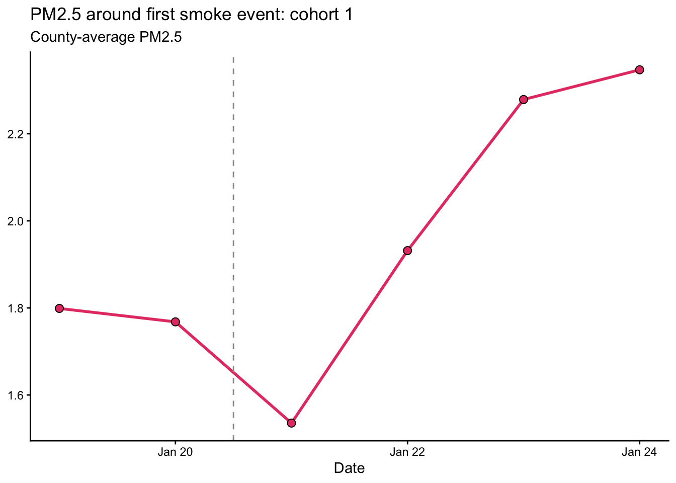

Treatment Group 2: February 19, 2016

library(ggplot2)

tg2_date <- as.Date("2016-02-19")
avg_tg_2 <- smoke[first_smoke_day == tg2_date,
                  .(avg_pm = mean(dietal_pm25)),
                  by = "date"]

ggplot(avg_tg_2[date > tg2_date - 2 & date < tg2_date + 5],
       aes(x = date, y = avg_pm)) +
  geom_line(color = "#E64173", linewidth = 1) +
  geom_point(shape = 21, fill = "#E64173", color = "black", size = 2.5) +
  geom_vline(xintercept = tg2_date + 0.5,
             linetype = "dashed", color = "grey60") +
  theme_classic() +
  labs(title = "PM2.5 around first smoke event: cohort 2",
       subtitle = "County-average PM2.5", x = "Date", y = NULL)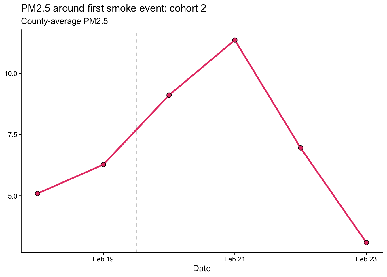

Both plots show clear spikes in PM2.5 at the treatment date, suggesting substantial smoke exposure effects.

Analysis with Never-Treated Controls

Step 1: Explore Kappa Trade-offs

R

to_never <- kappa_trade_offs(
  data = smoke,
  time_var = "date",
  unit_var = "fips",
  adopt_var = "first_smoke_day",
  kappa_pre_range = seq(2, 4, by = 1),
  kappa_post_range = seq(0, 4, by = 1),
  control_type = "never_treated"
)

# View the trade-offs
head(to_never)
#>    kappa_pre kappa_post n_sub_exp n_unidentified_sub_exp n_event_times n_obs
#> 1:         2          0         2                      0             3   609
#> 2:         2          1         2                      0             4   812
#> 3:         2          2         2                      0             5  1015
#> 4:         2          3         2                      0             6  1218
#> 5:         2          4         2                      0             7  1421
#> 6:         3          0         2                      0             4   812
#>    total_treated_obs total_control_obs avg_treated_per_period
#> 1:               549                60                    183
#> 2:               732                80                    183
#> 3:               915               100                    183
#> 4:              1098               120                    183
#> 5:              1281               140                    183
#> 6:               732                80                    183
#>    avg_control_per_period sd_treated_per_period sd_control_per_period
#> 1:                     20                     0                     0
#> 2:                     20                     0                     0
#> 3:                     20                     0                     0
#> 4:                     20                     0                     0
#> 5:                     20                     0                     0
#> 6:                     20                     0                     0
#>    adoption_times_str
#> 1:       16820, 16850
#> 2:       16820, 16850
#> 3:       16820, 16850
#> 4:       16820, 16850
#> 5:       16820, 16850
#> 6:       16820, 16850

Stata

* Explore kappa trade-offs with never-treated controls
stacked use smoke, clear
stacked kappa, time(date) unit(fips) adopt(first_smoke_day) ///
    kpre(2/4) kpost(0/4) controltype(never)
matrix list r(table)

This table shows how different kappa choices affect sample size, number of cohorts included, and the balance between treated and control observations.

Step 2: Build the Stack

R

stackdt_never <- build_stack(
  data = smoke,
  time_var = "date",
  unit_var = "fips",
  adopt_var = "first_smoke_day",
  kappa_pre = 2,
  kappa_post = 4,
  control_type = "never_treated"
)

# View the stacked data structure
head(stackdt_never[, .(fips, date, first_smoke_day,
                       sub_exp, event_time, treat, post, q_weight)])
#>     fips  date first_smoke_day sub_exp event_time treat post  q_weight
#> 1: 33001 16818              NA   16820         -2     0    0 0.3606557
#> 2: 33001 16819              NA   16820         -1     0    0 0.3606557
#> 3: 33001 16820              NA   16820          0     0    1 0.3606557
#> 4: 33001 16821              NA   16820          1     0    1 0.3606557
#> 5: 33001 16822              NA   16820          2     0    1 0.3606557
#> 6: 33001 16823              NA   16820          3     0    1 0.3606557

Stata

* Build the stack with never-treated controls (kpre=2, kpost=4)
stacked use smoke, clear
stacked build, time(date) unit(fips) adopt(first_smoke_day) ///
    kpre(2) kpost(4) controltype(never)

list fips date first_smoke_day sub_exp event_time treat post q_weight in 1/6

Step 3: Pooled Event Study

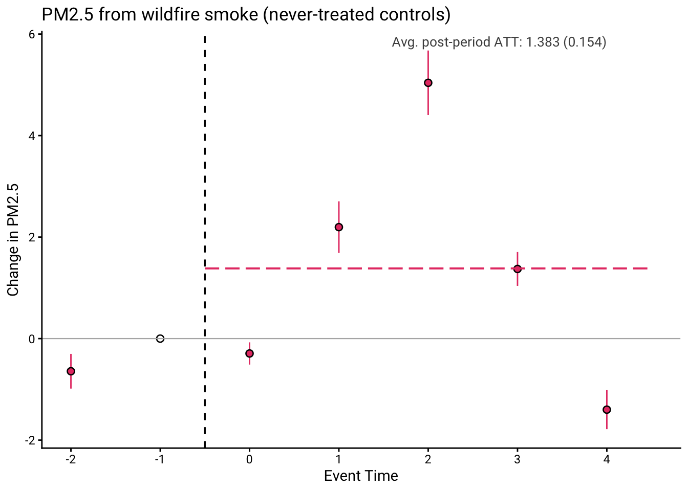
stackreg() fits the stacked regression (Q-weighted by default), and stack_plot() draws the event study in the house style: the corrective estimate in the highlight color, an open circle at the reference period, and the average post-period ATT as a dashed reference line.

R

model_never <- stackreg(
  stack_data = stackdt_never,
  outcome_var = "dietal_pm25",
  cluster_var = "fips",
  ref_period = -1
)

stack_plot(
  model_never,
  title = "PM2.5 from wildfire smoke (never-treated controls)",
  ylab = "Change in PM2.5"
)

Stata

* Q-weighted event study and coefficient plot
stacked reg dietal_pm25, cluster(fips) ref(-1)
stacked plot, title("PM2.5 from wildfire smoke (never-treated controls)")

Step 4: Cohort-Specific Event Studies

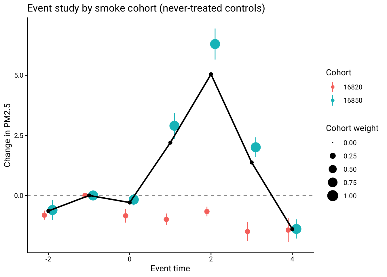
stackreg(by_group = TRUE) fits each adoption cohort separately. stack_plot(combine = "overlay") overlays the cohorts — point area is proportional to each cohort’s aggregation weight — with the pooled estimate as the solid black reference series. (The two smoke cohorts are the January 20 and February 19, 2016 events.)

R

groups_never <- stackreg(
  stack_data = stackdt_never,
  outcome_var = "dietal_pm25",
  cluster_var = "fips",
  ref_period = -1,
  by_group = TRUE
)

stack_plot(
  groups_never,
  combine = "overlay",
  title = "Event study by smoke cohort (never-treated controls)",
  ylab = "Change in PM2.5"
)

Stata

* Per-cohort event studies, overlaid with the pooled estimate
stacked reg dietal_pm25, cluster(fips) ref(-1) bygroup
stacked plot, bygroup combine(overlay) ///
    title("Event study by smoke cohort (never-treated controls)")

Step 5: Q-Weighted Outcome Levels

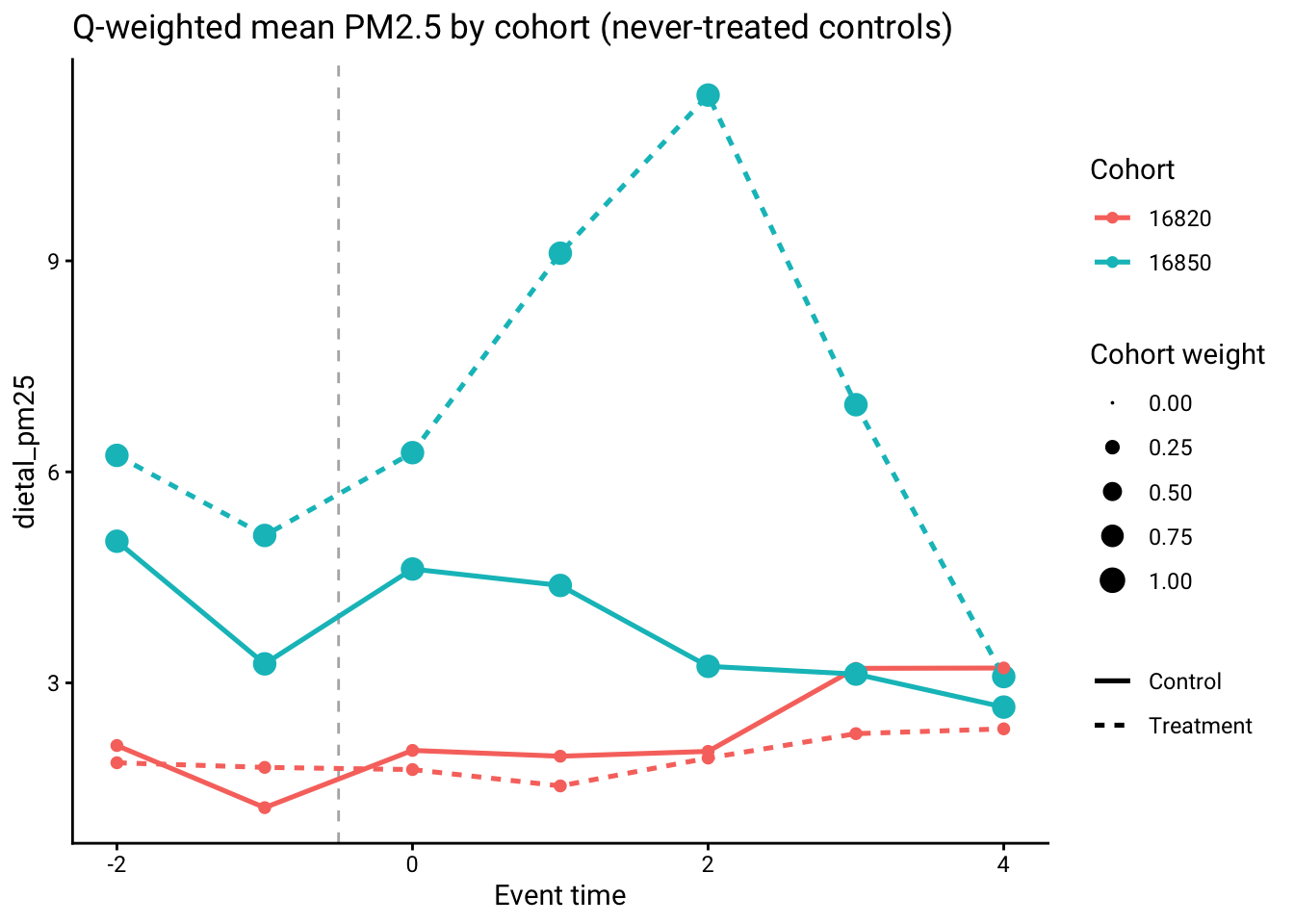
stack_plot_levels() shows the Q-weighted mean outcome for treated and control units at each event time — the levels behind the coefficients above. With by_group = TRUE the cohorts are overlaid.

R

stack_plot_levels(
  stackdt_never,
  outcome_var = "dietal_pm25",
  by_group = TRUE,
  combine = "overlay",
  title = "Q-weighted mean PM2.5 by cohort (never-treated controls)"
)

Stata

* Q-weighted mean outcome levels by cohort
stacked levels dietal_pm25, plot bygroup

Step 6: Timing-Group Decomposition

stack_summary() assembles the per-cohort static ATTs, each cohort’s precision and corrective weights, and the two aggregation identities in one place. The precision-weighted aggregate equals the unweighted stacked TWFE; the corrective-weighted aggregate equals the Q-weighted stacked TWFE (the target ATT). Their gap is summarized by the design divergence D.

R

sm_never <- stack_summary(
  stackdt_never,
  outcome_var = "dietal_pm25",
  cluster_var = "fips",
  model = "att"
)

knitr::kable(
  fmt_summary(sm_never),
  caption = "Static ATT by smoke cohort (never-treated controls)"
)

Static ATT by smoke cohort (never-treated controls)

Cohort	N obs	Treated units	Precision wt	Corrective wt	ATT	SE
2016-01-20	301	33	0.45	0.18	-0.680	0.116
2016-02-19	1120	150	0.55	0.82	2.229	0.122
Total	1421	183	1.00	1.00	1.705	0.108

knitr::kable(
  fmt_reconcile(sm_never),
  caption = "Aggregation identities and design divergence"
)

Aggregation identities and design divergence

Quantity	Value
Unweighted stacked TWFE (precision weights)	0.920
Q-weighted stacked TWFE (corrective weights)	1.705
Design divergence D	0.540

Stata

* Timing-group decomposition: per-cohort ATTs, weights, and the
* precision-vs-corrective reconciliation
stacked summary dietal_pm25, cluster(fips) model(att)

Analysis with Both Control Types

Now repeat the workflow using both never-treated and not-yet-treated units as controls.

Step 1: Build the Stack

R

stackdt_both <- build_stack(
  data = smoke,
  time_var = "date",
  unit_var = "fips",
  adopt_var = "first_smoke_day",
  kappa_pre = 2,
  kappa_post = 4,
  control_type = "both"
)

# Compare sample sizes
cat("Never-treated only:", nrow(stackdt_never), "observations\n")
#> Never-treated only: 1421 observations
cat("Both control types:", nrow(stackdt_both), "observations\n")
#> Both control types: 2471 observations

Stata

* Build the stack with both control types (kpre=2, kpost=4)
stacked use smoke, clear
stacked build, time(date) unit(fips) adopt(first_smoke_day) ///
    kpre(2) kpost(4) controltype(both)
display "Both control types: " r(n_obs) " observations"

Including not-yet-treated controls increases the number of control observations: here the second cohort serves as a not-yet-treated control for the first cohort’s sub-experiment.

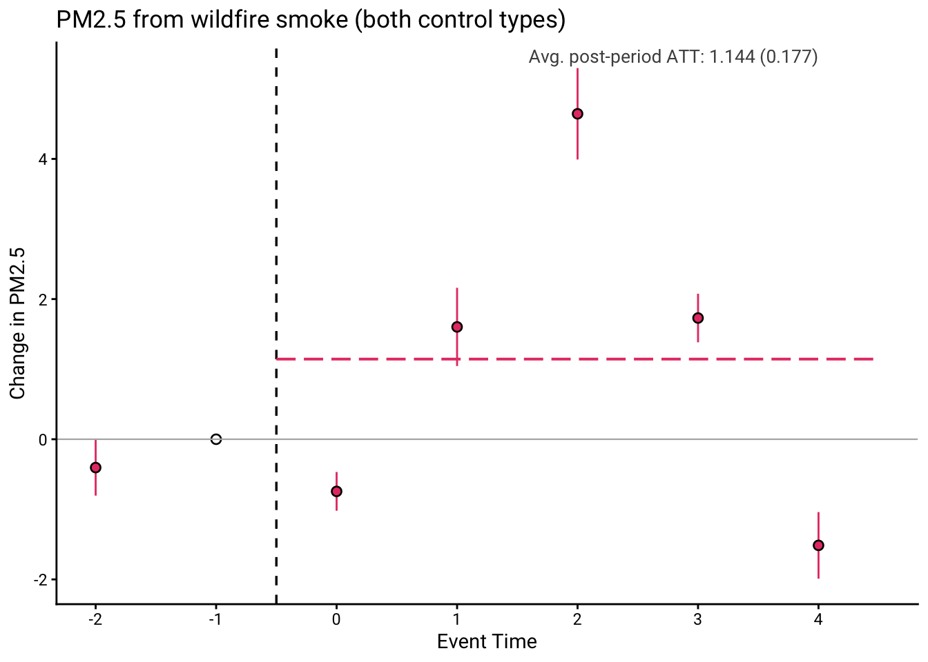
Step 2: Pooled Event Study

R

model_both <- stackreg(
  stack_data = stackdt_both,
  outcome_var = "dietal_pm25",
  cluster_var = "fips",
  ref_period = -1
)

stack_plot(
  model_both,
  title = "PM2.5 from wildfire smoke (both control types)",
  ylab = "Change in PM2.5"
)

Stata

* Q-weighted event study and coefficient plot
stacked reg dietal_pm25, cluster(fips) ref(-1)
stacked plot, title("PM2.5 from wildfire smoke (both control types)")

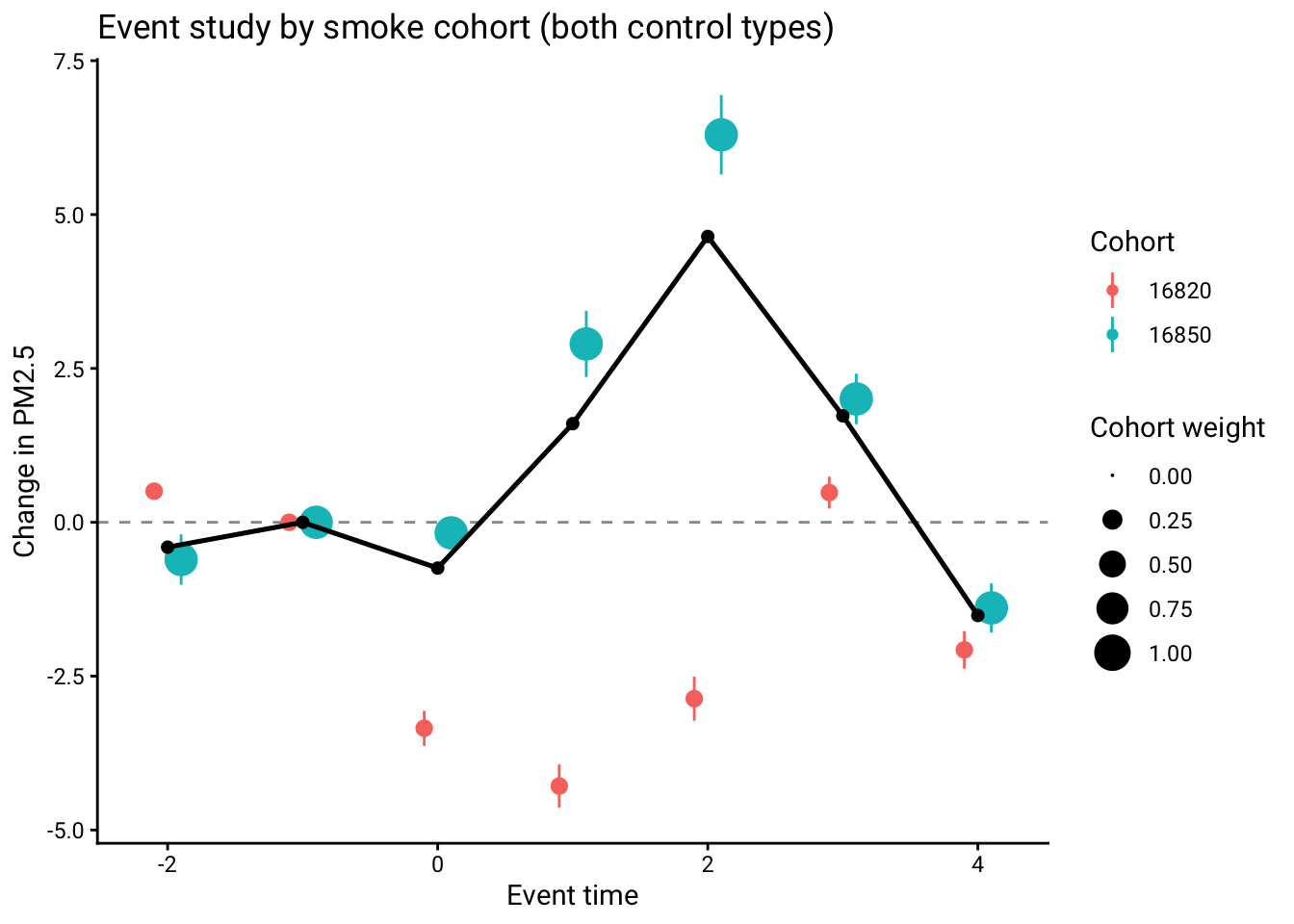
Step 3: Cohort-Specific Event Studies and Levels

R

groups_both <- stackreg(
  stack_data = stackdt_both,
  outcome_var = "dietal_pm25",
  cluster_var = "fips",
  ref_period = -1,
  by_group = TRUE
)

stack_plot(
  groups_both,
  combine = "overlay",
  title = "Event study by smoke cohort (both control types)",
  ylab = "Change in PM2.5"
)

Stata

* Per-cohort event studies, overlaid with the pooled estimate
stacked reg dietal_pm25, cluster(fips) ref(-1) bygroup
stacked plot, bygroup combine(overlay) ///
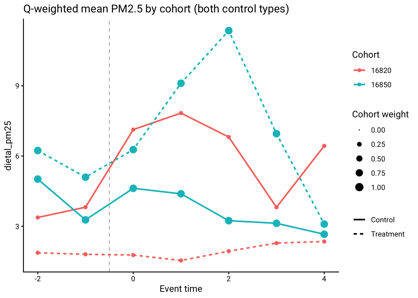
    title("Event study by smoke cohort (both control types)")

R

stack_plot_levels(
  stackdt_both,
  outcome_var = "dietal_pm25",
  by_group = TRUE,
  combine = "overlay",
  title = "Q-weighted mean PM2.5 by cohort (both control types)"
)

Stata

* Q-weighted mean outcome levels by cohort
stacked levels dietal_pm25, plot bygroup

Step 4: Timing-Group Decomposition

R

sm_both <- stack_summary(
  stackdt_both,
  outcome_var = "dietal_pm25",
  cluster_var = "fips",
  model = "att"
)

knitr::kable(
  fmt_summary(sm_both),
  caption = "Static ATT by smoke cohort (both control types)"
)

Static ATT by smoke cohort (both control types)

Cohort	N obs	Treated units	Precision wt	Corrective wt	ATT	SE
2016-01-20	1351	33	0.745	0.18	-2.670	0.135
2016-02-19	1120	150	0.255	0.82	2.229	0.122
Total	2471	183	1.000	1.00	1.346	0.165

knitr::kable(
  fmt_reconcile(sm_both),
  caption = "Aggregation identities and design divergence"
)

Aggregation identities and design divergence

Quantity	Value
Unweighted stacked TWFE (precision weights)	-1.420
Q-weighted stacked TWFE (corrective weights)	1.346
Design divergence D	1.129

Stata

* Timing-group decomposition with both control types
stacked summary dietal_pm25, cluster(fips) model(att)

Comparing Control Type Choices

The pooled Q-weighted ATT (with clustered standard errors) is stable across the two control-group choices:

knitr::kable(
  data.frame(
    `Control group` = c("Never-treated only", "Both control types"),
    `Pooled ATT` = round(c(sm_never$pooled$estimate, sm_both$pooled$estimate), 3),
    SE = round(c(sm_never$pooled$se, sm_both$pooled$se), 3),
    check.names = FALSE
  ),
  caption = "Pooled Q-weighted ATT by control-group choice"
)

Pooled Q-weighted ATT by control-group choice

Control group	Pooled ATT	SE
Never-treated only	1.705	0.108
Both control types	1.346	0.165

Summary

This applied example ran the full workflow through the package API:

1. Data exploration: raw treatment timing and outcomes
2. Kappa trade-offs: kappa_trade_offs() for parameter choices
3. Stack construction: build_stack() with different control types
4. Estimation and event studies: stackreg() + stack_plot()
5. Cohort heterogeneity: stackreg(by_group = TRUE) + stack_plot() overlay, stack_plot_levels(), and the stack_summary() decomposition
6. Reconciliation: stack_summary() confirms that the precision- and corrective-weighted aggregates match the unweighted and Q-weighted stacked TWFE coefficients

The smoke exposure example shows clear treatment effects on PM2.5, with both control-type choices yielding similar conclusions. The choice between control types depends on your research design and the plausibility of parallel trends for each control group.