Paper

Here’s a link to the NBER Working paper version. An updated version is coming soon!

Stacked difference-in-differences estimators handle staggered adoption designs by building a clean sub-experiment around each adoption event and pooling them in one regression. Stacking removes the “forbidden” comparisons that bias two-way fixed effects, but it does not address a second problem: aggregation. The unweighted stacked fixed-effects regression used in applied work weights each sub-experiment by the precision of its own difference-in-differences (the inverse of the familiar two-sample variance) rather than by its share of treated units. Under treatment-effect heterogeneity the two weighting schemes can disagree enough to flip the sign of the estimate; in three canonical applications — unilateral divorce, naloxone access laws, and the ACA Medicaid expansion — the two answers on the same data range from indistinguishable to completely different. We derive corrective sample weights, computable from the stacked data itself, under which a single weighted regression identifies a transparent target: a trimmed aggregate ATT whose composition is fixed over event time, so that estimated dynamics and pre-trends reflect treatment effects rather than composition. The same construction delivers population-weighted, survey-weighted, and propensity-score-weighted aggregates. Companion R and Stata packages implement the method at any scale.

Exhibits

The five exhibits below are the paper’s current figures and tables. The two tables (Exhibits 4 and 5) are typeset natively; every cell mirrors the manuscript, including the precision weights \(w^S_g\), the corrective weights \(w^T_g\), the treated and control masses \(m^D_g\) and \(m^C_g\), and the design divergence \(D\).

Exhibit 1 — Compositional balance

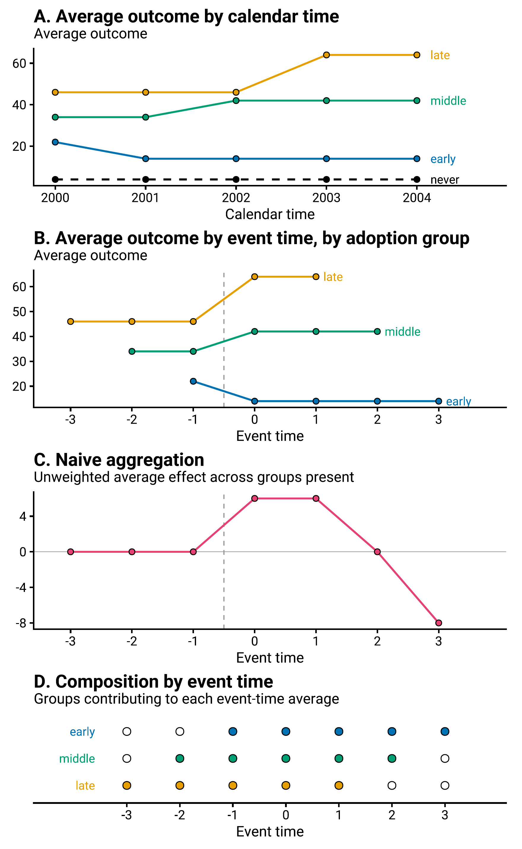
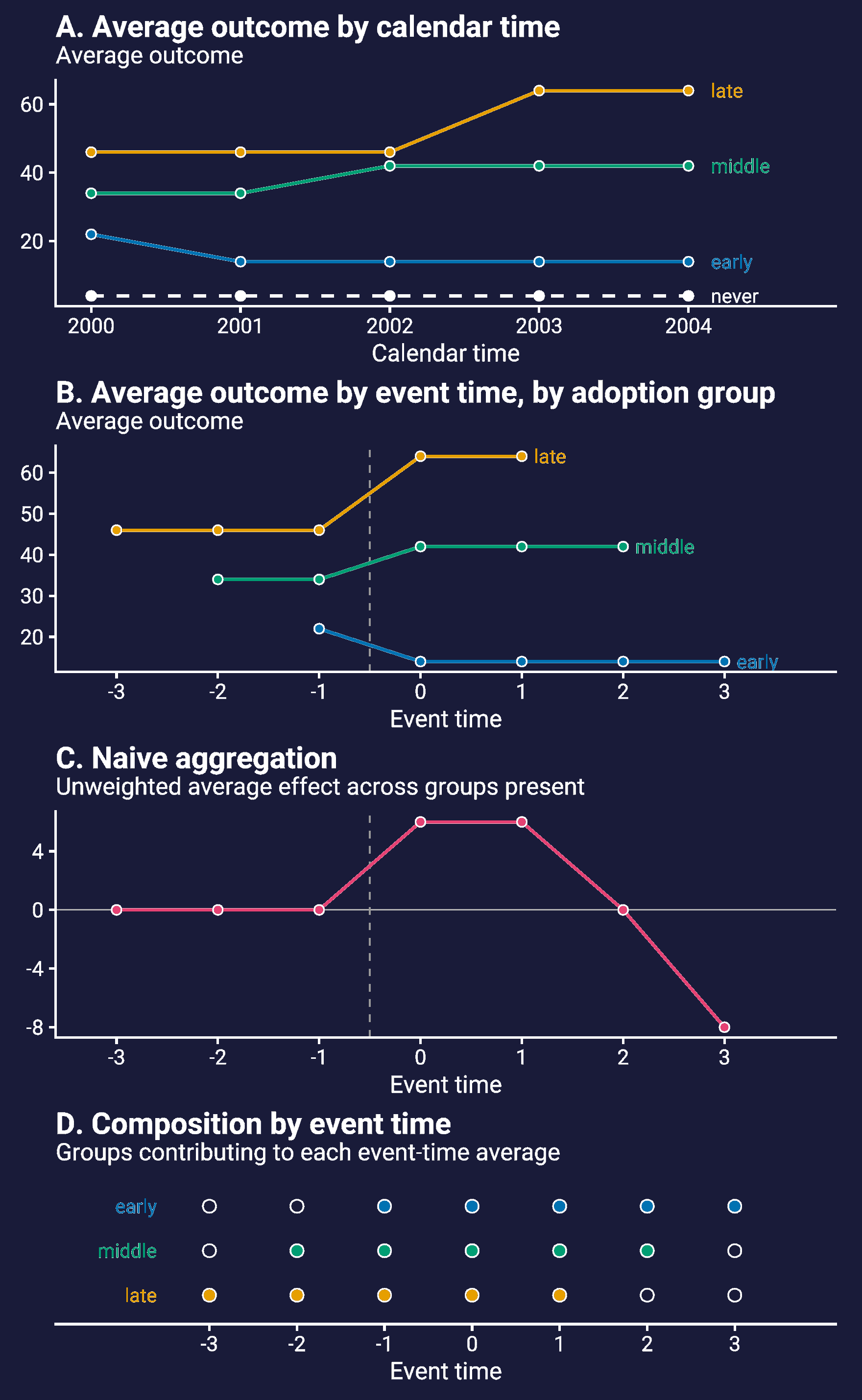
Exhibit 2 — Simulated designs

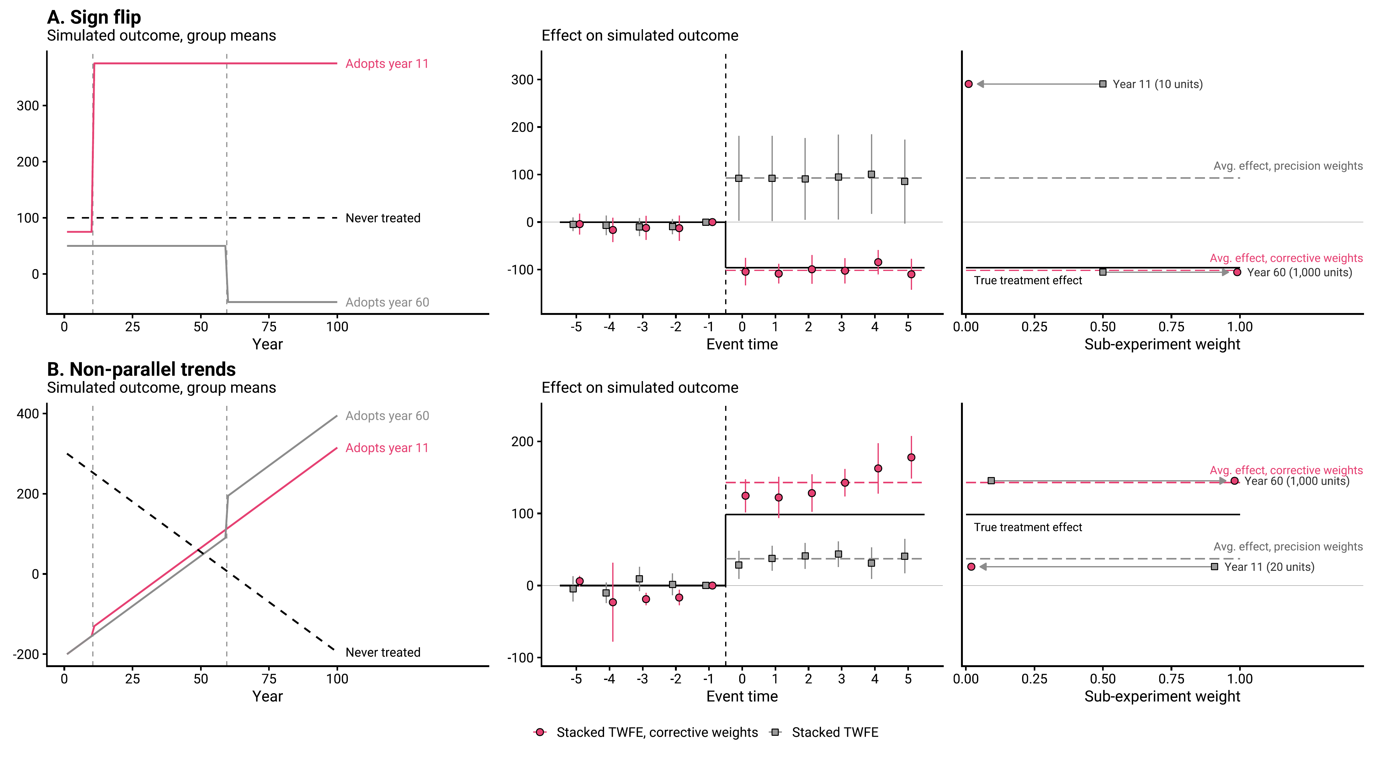
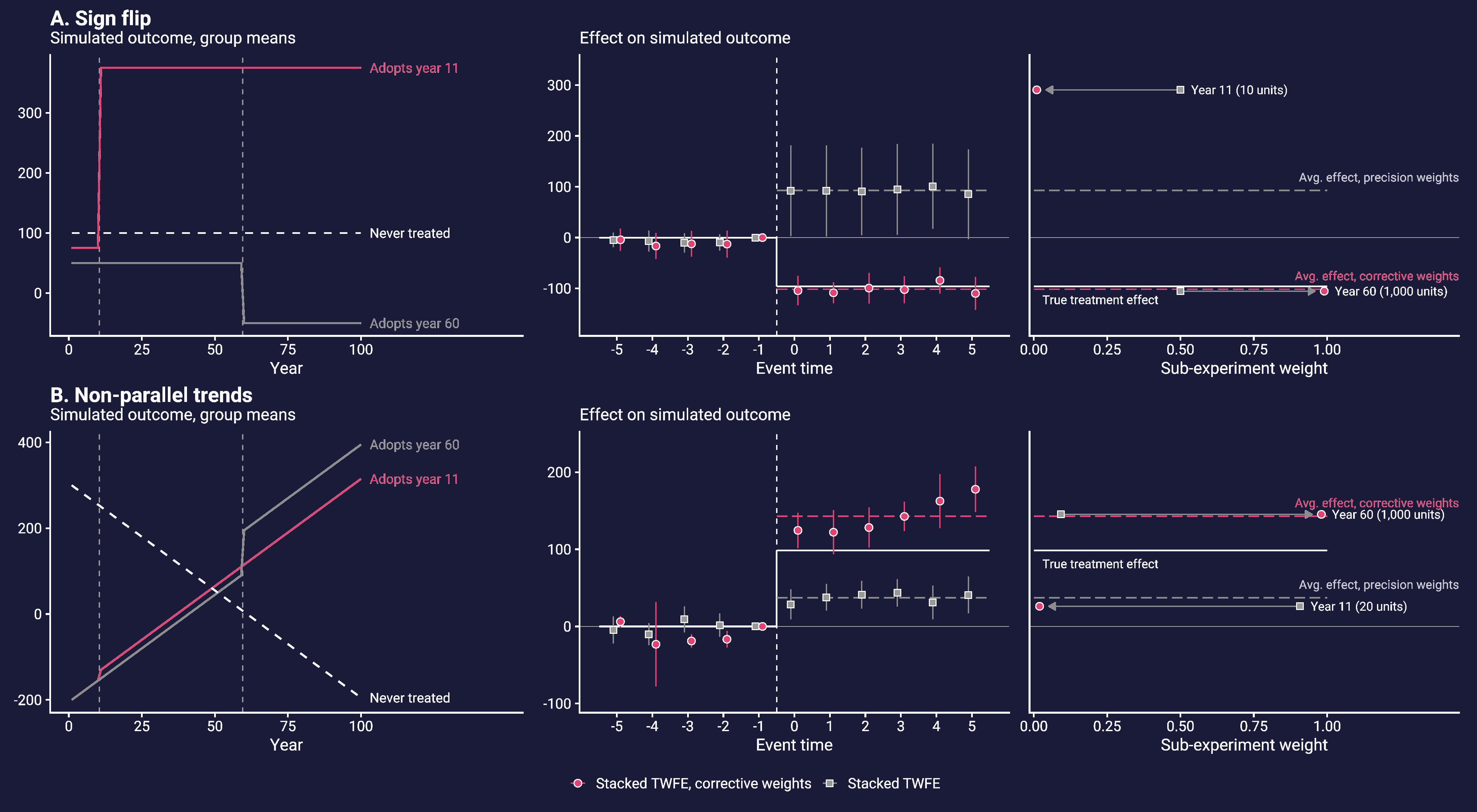
Exhibit 3 — Real-data applications

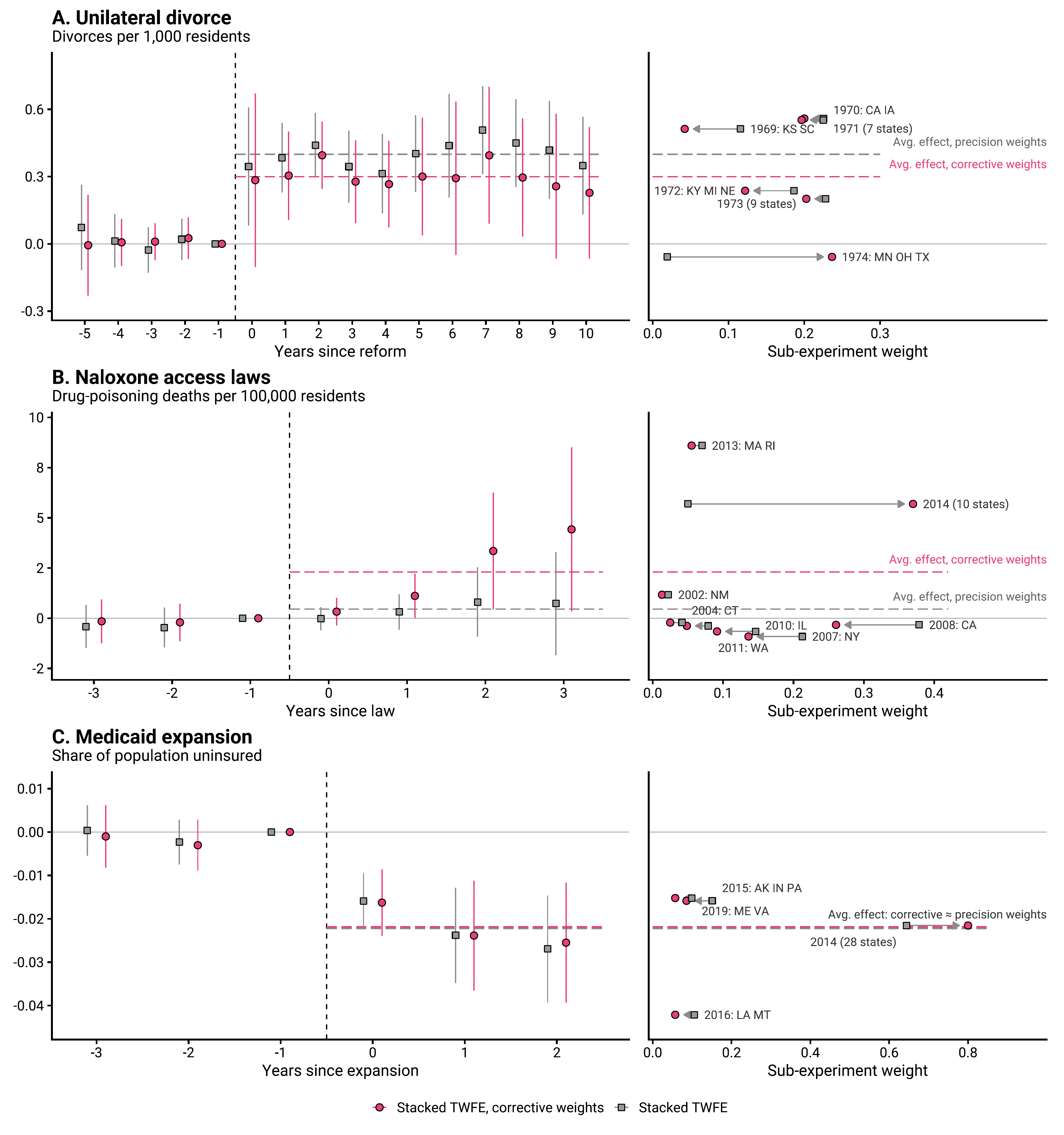
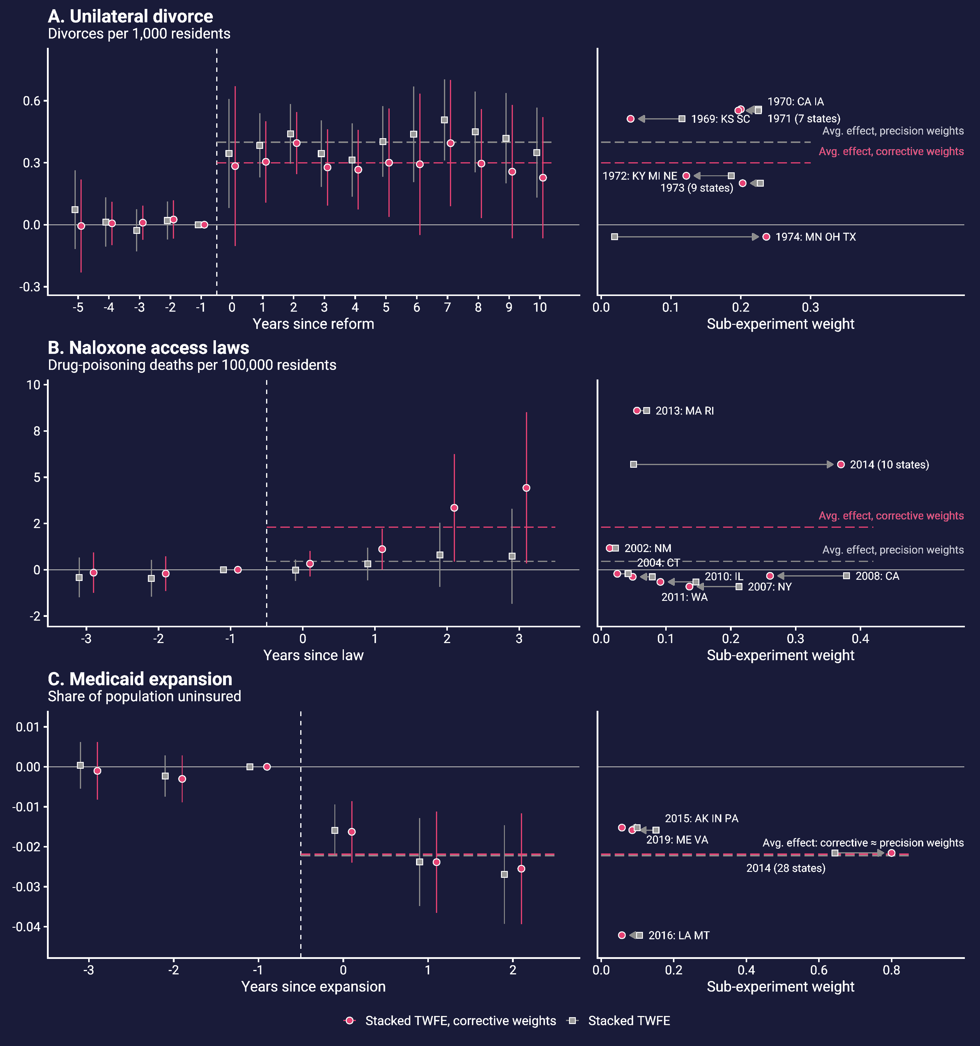
Exhibit 3. Three applications on the same data — unilateral divorce, naloxone access laws, and the ACA Medicaid expansion.

Exhibit 4 — Timing-group decomposition of the stacked estimates

	Stacked	Stacked	Sub-group	Treated	Control	Precision	Corrective
	w/ corr.	w/o corr.	ATT /	mass	mass	weight	weight
	weights	weights	difference	(m^D_g)	(m^C_g)	(w^S_g)	(w^T_g)
Panel 1: Simulated examples
A. Sign flip
Aggregate ATT	−101***	93**	−194	(=291(0.01-0.50)-105(0.99-0.50))
	(12.14)	(44.47)
	[12.10]
Sub-group ATTs
Adopts year 11			291	10	1010	0.50	0.01
Adopts year 60			−105	1000	10	0.50	0.99
(D) (design divergence)			0.98	(=\|0.50-0.01\|+\|0.50-0.99\|)
B. Non-parallel trends
Aggregate ATT	143***	37***	106	(=26(0.02-0.91)+145(0.98-0.09))
	(5.73)	(8.99)
	[5.71]
Sub-group ATTs
Adopts year 11			26	20	1002	0.91	0.02
Adopts year 60			145	1000	2	0.09	0.98
(D) (design divergence)			1.78	(=\|0.91-0.02\|+\|0.09-0.98\|)
Panel 2: Real-data examples
A. Unilateral divorce (divorces per 1,000 residents)
Aggregate ATT	0.30***	0.40***	−0.10
	(0.113)	(0.073)
	[0.069]
Sub-group ATTs
1969			0.51	4.8	23.4	0.12	0.04
1970			0.56	22.8	11.8	0.23	0.20
1971			0.55	22.4	11.9	0.23	0.20
1972			0.24	13.9	11.9	0.19	0.12
1973			0.20	23.1	11.9	0.23	0.20
1974			−0.06	26.9	0.7	0.02	0.24
(D) (design divergence)			0.43
B. Naloxone access laws (drug-poisoning deaths per 100,000)
Aggregate ATT	2.30**	0.46	1.85
	(1.085)	(0.673)
	[0.477]
Sub-group ATTs
2002			1.17	1.9	282.3	0.02	0.01
2004			−0.22	3.5	268.2	0.04	0.02
2007			−0.91	19.1	227.6	0.21	0.14
2008			−0.33	36.6	223.4	0.38	0.26
2010			−0.66	12.8	219.8	0.15	0.09
2011			−0.38	6.8	170.6	0.08	0.05
2013			8.60	7.8	23.3	0.07	0.06
2014			5.69	52.0	4.5	0.05	0.37
(D) (design divergence)			0.64
C. Medicaid expansion (share of population uninsured)
Aggregate ATT	−0.022***	−0.022***	0.000
	(0.0056)	(0.0048)
	[0.0055]
Sub-group ATTs
2014			−0.022	28	18	0.64	0.80
2015			−0.016	3	18	0.15	0.09
2016			−0.042	2	18	0.11	0.06
2019			−0.015	2	11	0.10	0.06
(D) (design divergence)			0.31

Exhibit 4. Timing-group decomposition of the stacked estimates. Each sub-panel decomposes the two stacked estimates into timing-group (sub-experiment) components at the example’s headline design; stacks include only identified sub-experiments. Sub-group ATTs are cohort-specific average post-period effects. For timing group (g), (m^D_g) and (m^C_g) are its treated and control masses — populations in millions where the estimator is population-weighted (the divorce and naloxone examples), unit counts otherwise. Precision weights (w^S_g) are the variance-efficient weights the non-corrective stacked TWFE implicitly applies; corrective weights (w^T_g) are the treated-share targets of the Q-weighted estimator; both follow from the masses: (w^S_g = ) and (w^T_g = m^D_g/_h m^D_h). The difference column reports the corrective-minus-precision aggregate ATT, which equals (_g _g (w^T_g - w^S_g)); Panel 1 writes this arithmetic out beside the difference (up to rounding), and the same identity applies in Panel 2. Standard errors are clustered on the original unit: parentheses are from the pooled interacted-FE model in both columns; brackets, under the corrective ATT only, are from the joint saturated (cohort-specific) model. Stars use the interacted-FE standard errors: * p (<) 0.1, ** p (<) 0.05, *** p (<) 0.01. (D=_g |w^S_g - w^T_g|) summarizes the design divergence.

Exhibit 5 — Monte Carlo evidence on inference in the Q-weighted stacked DID

	(G)	True ()	SD ()	Average standard error			Rejection rate ((= .05))
				Sat, g	FE, g	FE, g()s	Sat, g	FE, g	FE, g()s	Wild, g
Panel A: Static aggregate ATT ((= -0.02))
Real common shocks	51	−0.020	0.0070	0.0075	0.0070	0.0065	0.046	0.061	0.084	0.064
Shocks removed	51	−0.020	0.0071	0.0069	0.0070	0.0065	0.061	0.057	0.080	0.054
Real common shocks	25	−0.020	0.0103	0.0107	0.0100	0.0092	0.059	0.071	0.089	0.066
Panel B: Event-study coefficients across cluster counts ((_e = -0.015 - 0.005e))
(e = 0)	25	−0.015	0.0066	0.0073	0.0067	0.0065	0.047	0.068	0.073	0.070
(e = 1)	25	−0.020	0.0103	0.0115	0.0102	0.0099	0.046	0.070	0.079	0.066
(e = 2)	25	−0.025	0.0116	0.0131	0.0116	0.0111	0.043	0.073	0.077	0.065
(e = 0)	51	−0.015	0.0049	0.0051	0.0047	0.0045	0.054	0.073	0.086	0.079
(e = 1)	51	−0.020	0.0074	0.0081	0.0072	0.0070	0.043	0.068	0.073	0.064
(e = 2)	51	−0.025	0.0083	0.0091	0.0081	0.0078	0.037	0.061	0.071	0.062
(e = 0)	100	−0.015	0.0032	0.0036	0.0033	0.0032	0.028	0.043	0.051	0.046
(e = 1)	100	−0.020	0.0049	0.0057	0.0051	0.0049	0.025	0.048	0.058	0.046
(e = 2)	100	−0.025	0.0055	0.0065	0.0057	0.0055	0.028	0.048	0.056	0.044
(e = 0)	500	−0.015	0.0014	0.0016	0.0015	0.0014	0.028	0.042	0.045	0.042
(e = 1)	500	−0.020	0.0022	0.0025	0.0023	0.0022	0.025	0.044	0.049	0.043
(e = 2)	500	−0.025	0.0025	0.0029	0.0025	0.0025	0.025	0.053	0.060	0.050

Exhibit 5. Monte Carlo evidence on inference in the Q-weighted stacked DID. Monte Carlo built on the Medicaid expansion application (51 states, annual uninsured rates, 2008–2021, ({pre}=3), ({post}=2)), so the error structures are the real ones. Each replication draws (G) states with replacement, keeping each state’s entire outcome path (and hence the real within-state dependence and real common time shocks), randomly assigns adoption timing using the application’s cohort mix (28 of 51 states in 2014, small later cohorts, 11 never treated) so that common trends holds by construction, adds a known treatment effect to treated-post outcomes, rebuilds the stack, and tests the Q-weighted estimate against the truth at (= .05). In Panel A the effect is static ((= -0.02)) and the test is on the average post-period ATT; “shocks removed” first demeans the outcome by calendar year, deleting the common shocks while keeping everything else. In Panel B the effect grows with event time ((_e = -0.015 - 0.005e)) and each post-period event-study coefficient is tested separately; resampling with replacement lets (G) exceed the 51 observed states while preserving the cohort mix and within-state dependence. “Sat” is the fully saturated specification and “FE” the interacted (unit and time by sub-experiment) specification — the two return identical point estimates, so bias (negligible everywhere) and SD () are common across tests. “g” clusters at the state level, “g()s” at state () sub-experiment; “Wild” is a restricted (null-imposed) wild cluster bootstrap-(t) (Rademacher weights, (B = 399)) on the interacted specification’s residuals, clustered at the state level. Panel A uses 2,000 replications per row (simulation standard error (.005) at a true rate of .05); Panel B uses 1,000 (simulation standard error (.007)).