Stacking, aggregation issues, and corrective weights

Stacked difference-in-differences is a transparent way to estimate treatment effects when units adopt treatment at different times. This page walks through the three ideas that make it work: the method (how the stack is built), the aggregation issue, and the correction.

Stacking

With staggered adoption, a standard two-way fixed effects (TWFE) regression pools every unit into one equation and lets already-treated units serve as controls for later-treated ones. Under effect heterogeneity that produces negative implicit weights and estimates that need not correspond to any treatment effect of interest.

Stacking replaces that single messy comparison with a set of clean ones. It is mechanically clean since any problematic comparison is omitted by design. For each adoption cohort (AKA timing-group) \(a\) we build a sub-experiment:

1. One cohort at a time. The treated group is the units that adopt in year \(a\).
2. Clean controls only. The control group is drawn from units that are not treated over the relevant window. This could be never-treated units, not-yet-treated units, or both. Already-treated units are never used as controls since the goal of stacking is to remove forbidden comparisons.
3. Align by event time. Calendar time is recentered on adoption, so \(\text{event\_time} = -1, 0, 1, \dots\) means the same thing in every sub-experiment.
4. A fixed event window. Fixing the event-window involves selecting two parameters, \(\kappa_{\text{pre}}\) and \(\kappa_{\text{post}}\). These set how many periods before and after adoption each sub-experiment spans. Cohorts too close to the edges of the panel to fill the window are dropped (see Compositional balance).

Stacking the sub-experiments and estimating one event-study regression gives a picture that by construction clean. Every comparison is between a treated cohort and an untreated cohort in the same calendar time. And each event-time period is observed in each stack, removing issues where compositional changes might masquerade as dynamic treatment effects in the aggreagation.

Aggregation issues

Here is the subtlety. Building a compositionally clean stack fixes many of the problems Goodman-Bacon pointed out related to negative-weights and forbidden comparisons. But it does not guarantee that a TWFE regression on the stacked data will actually return the average effect you care about.

The reason is that the sub-experiments differ in size. A pooled regression on the stack implicitly weights each sub-experiment by its share of the treatment variance, which depends on how many treated and control observations it contributes, not by its share of the treated units. When the ratio of treated to control units differs across cohorts, the regression averages the treated-group trend and the control-group trend using different weights. Even if parallel trends holds inside every sub-experiment, that mismatch biases the pooled coefficient.

Things go wrong when cohorts differ in their treatment effects. The pooled stacked estimate biases toward whichever cohorts happen to carry the most variance. This can even flip the sign of the treatment effect estimate.(see our sign flip example).

How far apart the two estimates can be is a property of the design alone — the D statistic — knowable before you look at a single outcome.

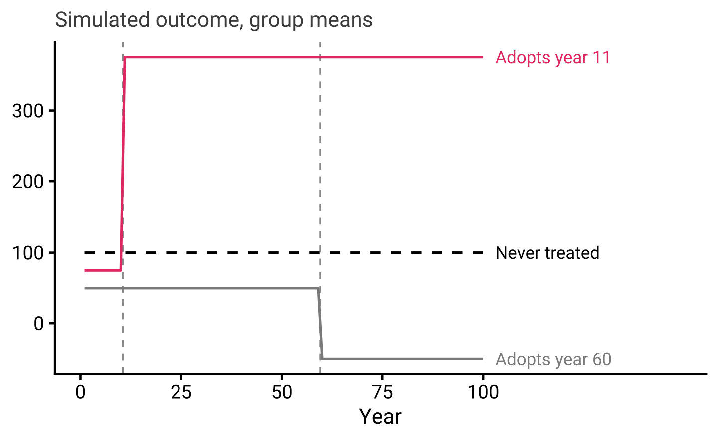
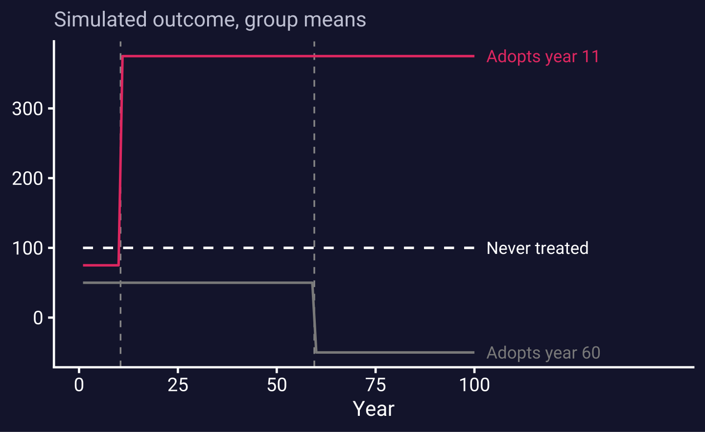
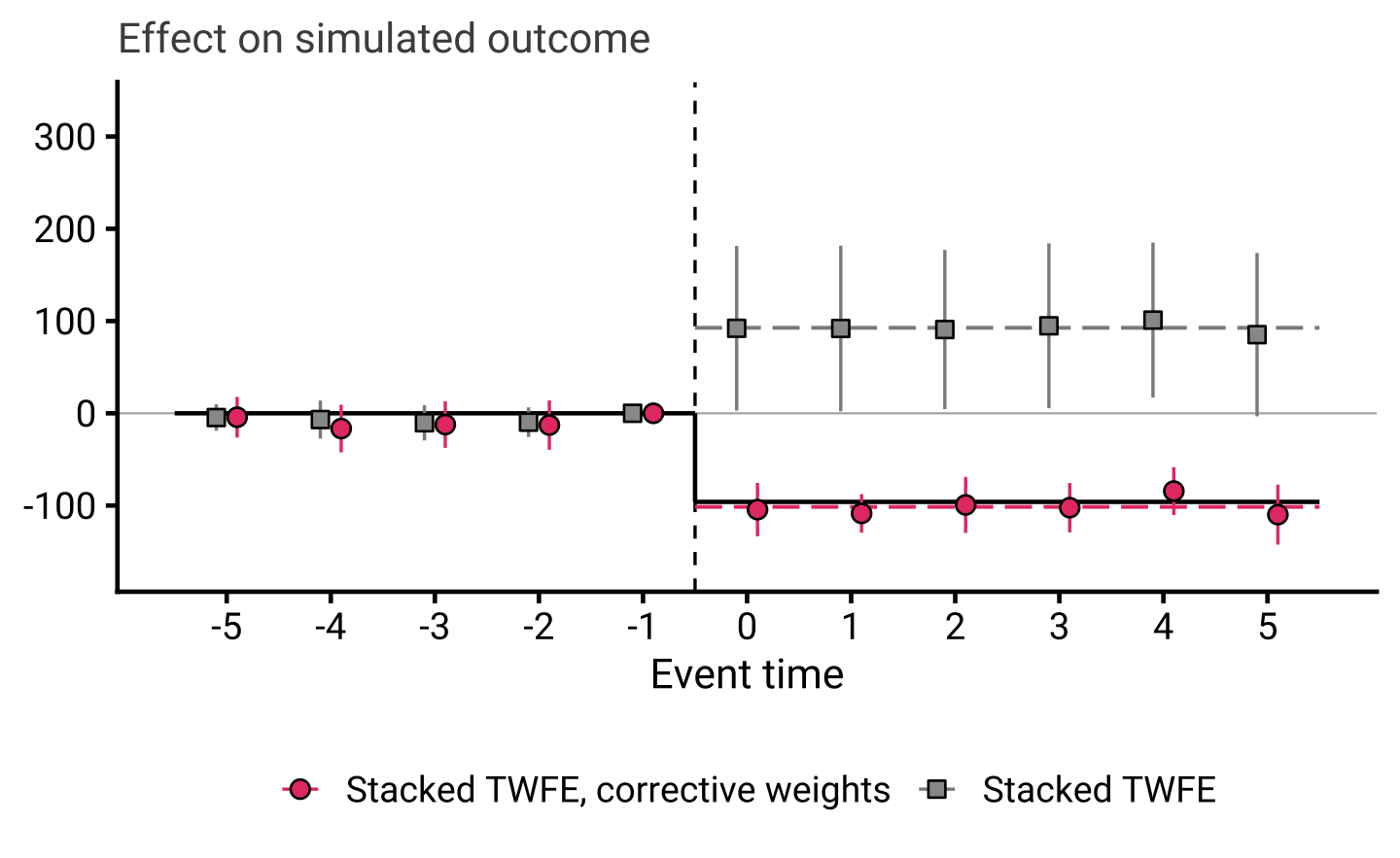
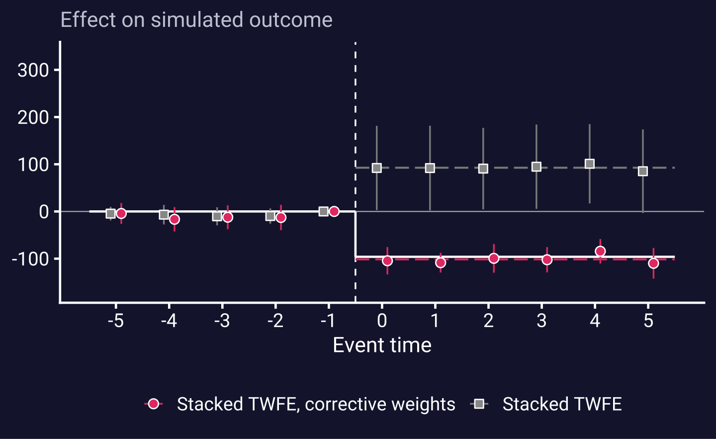
The site’s running example makes this concrete. We simulate data showing a sign-flip. Here a small cohort adopting in year 11 has a large positive effect (+300); a large cohort adopting in year 60 has a negative effect (−100). The treated-unit-weighted truth is negative, about −96, but the unweighted stacked TWFE is pulled above zero by the small, high-variance early cohort.

• 10 groups adopt in year 11 with a large positive effect (300)
• 1,000 groups adopt in year 60 with a negative effect (−100)

The simple unit-weighted average should clearly be negative (-96 \(~ = \frac{300\times 10 -100\times 1000}{10 + 1000}\)).

But a plain stacked TWFE regression without-corrective weights returns 93. Not only is this the wrong answer it is the wrong sign.

Raw group means — the small year-11 cohort jumps up, the large year-60 cohort drops, the never-treated units are flat (presented without error simply for a legible picture):

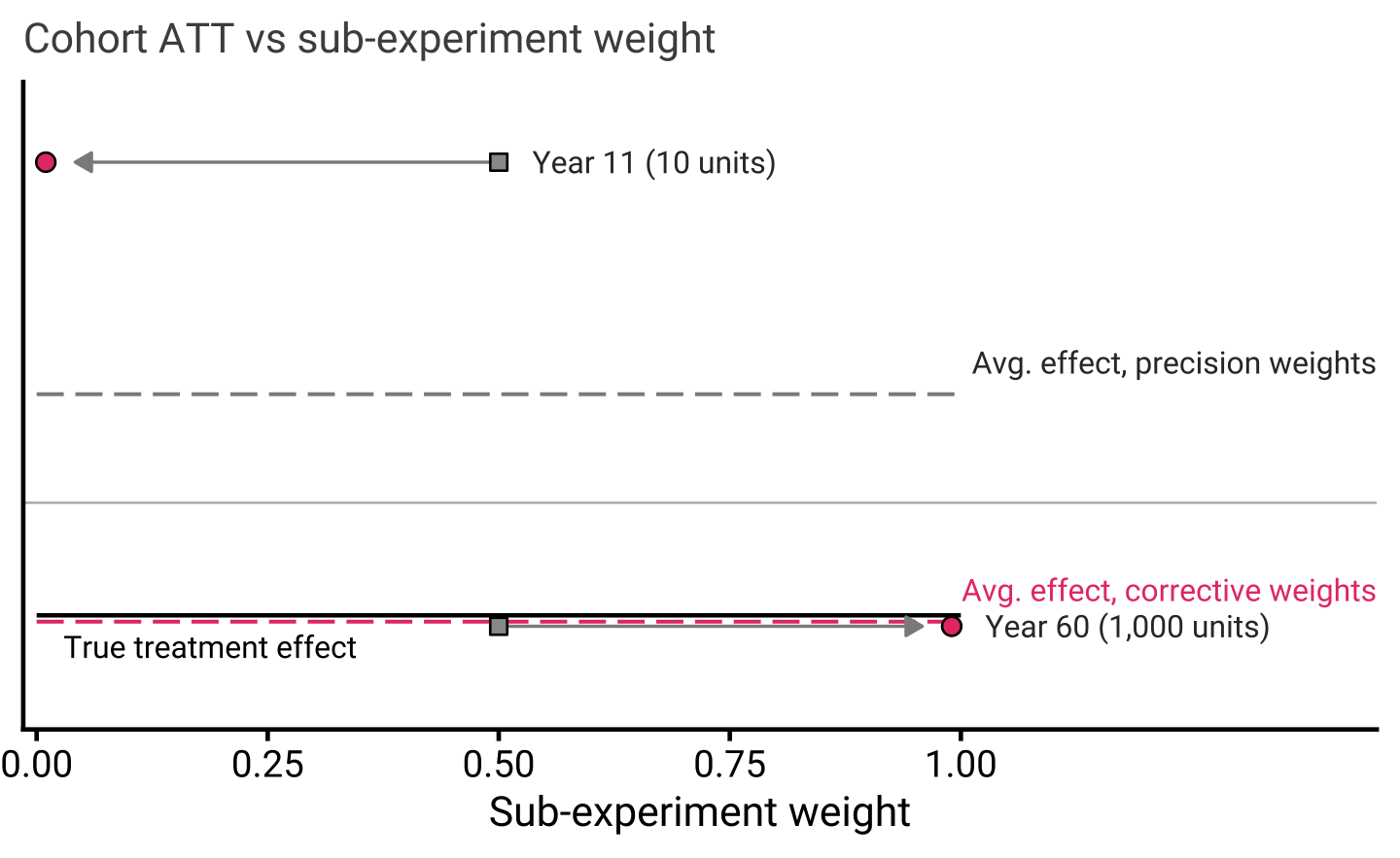
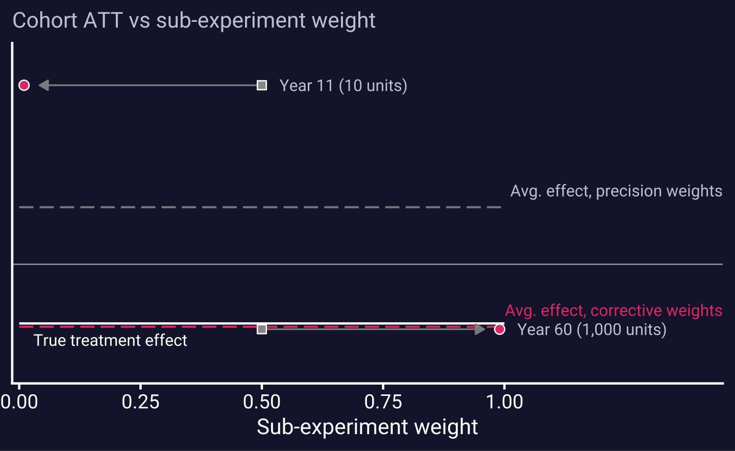
Each cohort’s ATT scattered against its sub-experiment weight without and without corrective weighting. We call the stacked TWFE without corrective-weights, precision weighting.

• Here the precision weights split the mass 50%/50%,
• while corrective weighting correclty loads 99% on the large negative cohort

Event studies for both estimators. Only the event-studies from stacked TWFE using corrective weights (pink) track the true ATT. The unweighted stacked TWFE (grey) sits on the wrong side of zero throughout:

Corrective weights

The fix is to weight the regression so that the same weighting scheme is applied to the treated and control groups. First fix the target. The default estimand is the treated-unit-weighted average effect: each cohort’s group-time ATT enters in proportion to its share of the treated units,

\[ \theta_{\kappa}^{e} \;=\; \sum_{a \in \Omega_{\kappa}} \operatorname{ATT}(a, a+e)\;\times\;\frac{N_a^{D}}{N_{\Omega_\kappa}^{D}}, \]

with the composition held fixed across event times \(e\), so movement in \(\theta_\kappa^e\) reflects genuine dynamics rather than a changing mix of cohorts.

The corrective-weights (Q-weights) make a weighted regression hit that target. Treated observations get weight 1. A control observation in sub-experiment \(a\) gets

\[ Q_a \;=\; \frac{N_a^{D}\,/\,N_{\Omega}^{D}}{N_a^{C}\,/\,N_{\Omega}^{C}}, \]

the ratio of the cohort’s treated share to its control share. This rescales each cohort’s controls so that treated and control trends are averaged with identical weights; the differential-weighting bias cancels, and the regression coefficients identify \(\theta_\kappa^e\). Cohorts that are over-represented among the controls relative to their treated mass get pulled down; under-represented cohorts get pushed up.

build_stack() computes q_weight for you, and stackreg() (R) / stacked reg (Stata) uses it automatically. On our running sign-flip example — ten units adopting in year 11, a thousand adopting in year 60, sharing one control pool — the control weights land far from 1:

R

source("assets/style-web.R")     # loads stacked, data.table, ggplot2
source("assets/sim-signflip.R")  # the paper's simulated sign-flip (running example)

sim   <- simulate_signflip()
stack <- build_stack(
  sim[, .(group_unit, year, adopt_year = time_treated, dep_var)],
  "year", "group_unit", "adopt_year",
  kappa_pre = KP, kappa_post = KQ,
  control_type = "both", weight_type = "unit_weights")

# Treated observations always carry weight 1; control weights vary by cohort.
# The large year-60 cohort has few controls of its own, so they are upweighted
# ~101x; the small year-11 cohort is swamped by controls, so its are pushed to 0.01.
stack[, .(mean_q_weight = round(mean(q_weight), 2)),
      by = .(treat, sub_exp)][order(treat, sub_exp)]

   treat sub_exp mean_q_weight
1:     0      11          0.01
2:     0      60        100.99
3:     1      11          1.00
4:     1      60          1.00

Stata

* Build the simulated sign-flip panel as on the worked-example page, then:
stacked build, time(year) unit(group_unit) adopt(adopt_year) ///
    kpre(5) kpost(5) controltype(both) weighttype(unit_weights)

* Treated observations carry weight 1; control weights vary by cohort
table treat sub_exp, statistic(mean q_weight)

Because the design is saturated in treatment status and event time, the Q-weighting also makes unit and time fixed effects redundant: the saturated specification and the canonical unit-by-cohort / time-by-cohort TWFE give identical point estimates.

Corrective weights will not always be consequential. They matter when cohorts are both unbalanced and heterogeneous; when they are not, it costs nothing. Real applications bear this out. In the paper we examine both unilateral divorce and naloxone access examples where the corrective and precision-weighted aggregates differ. On the other hand, we also example a Medicaid expansion example where the corrective weights do little to change the average treatment effect. In this case, the treated cohorts happen to have similar effects, so the two post-period ATTs land within a hair of each other (\(-0.0219\) vs \(-0.0222\)). The simulated running example above isolates a consequential case.

To help diagnose the potential for issues before estimating treatment effects, we also provide a diagnostic divergence statistic, which will give some idea about how much difference there is between precision- and corrective-weights.

Where to next

• Compositional balance: showing how compositional balance can masquerade as dynamic treatment effects. Also introducing a D statistic which can help diagnose when naive and corrected estimates might diverge.
• Static example using simulated data: using a tiny dataset where naive stacked TWFE gets the sign wrong.
• Interactive app: move the pieces with sliders and watch the estimators diverge.
• Paper: the working paper.