Stacked difference-in-differences works because every comparison is between a treated cohort and clean controls at the same event time. Two things can quietly break that clean picture: the mix of cohorts can change across event time, and the balance of treated to control units can differ across cohorts. This page explains both, and the single design diagnostic — the divergence statistic D — that tells you, before you look at any outcome, how much the naive and corrected estimates can disagree.
Composition changing across event time
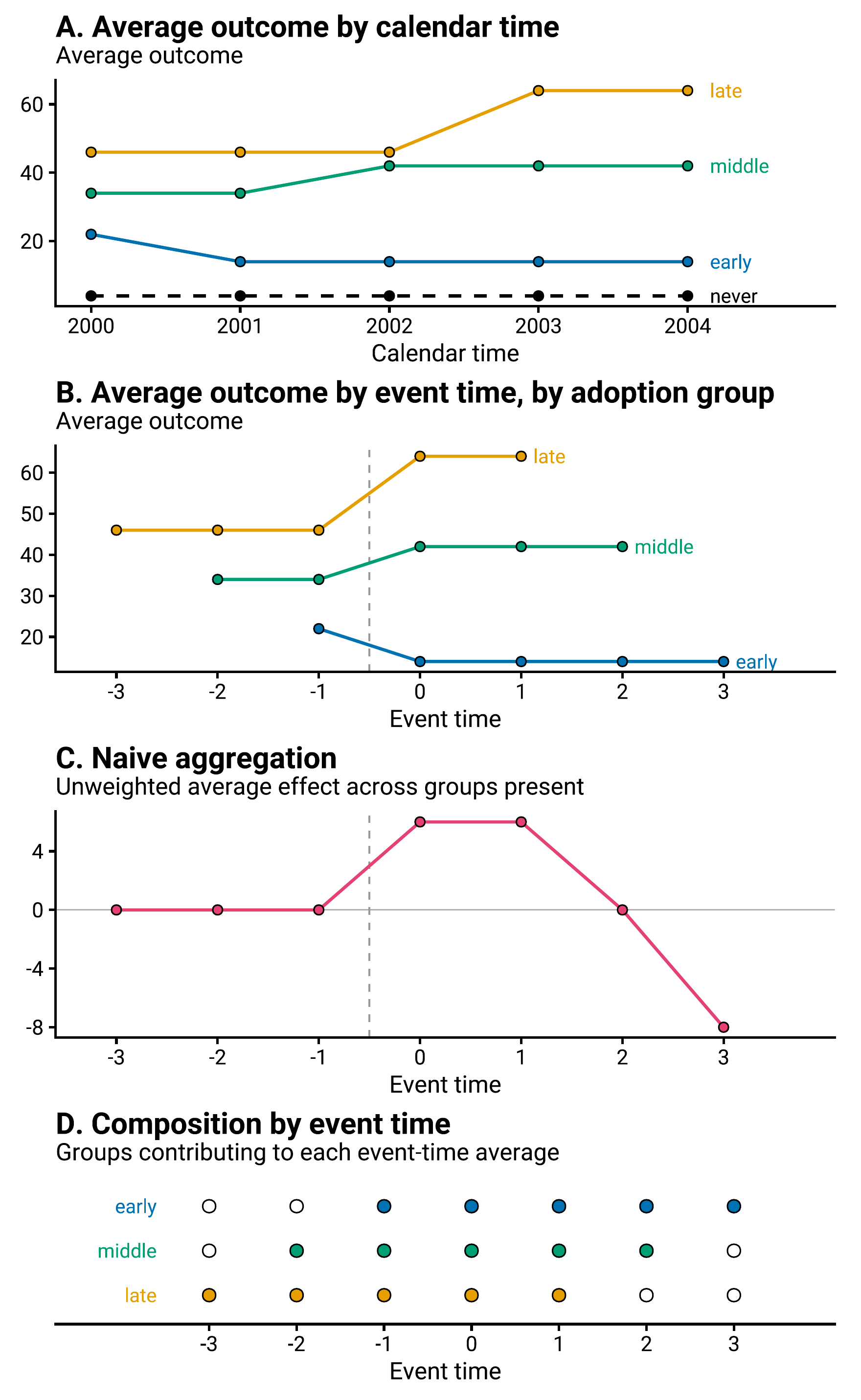
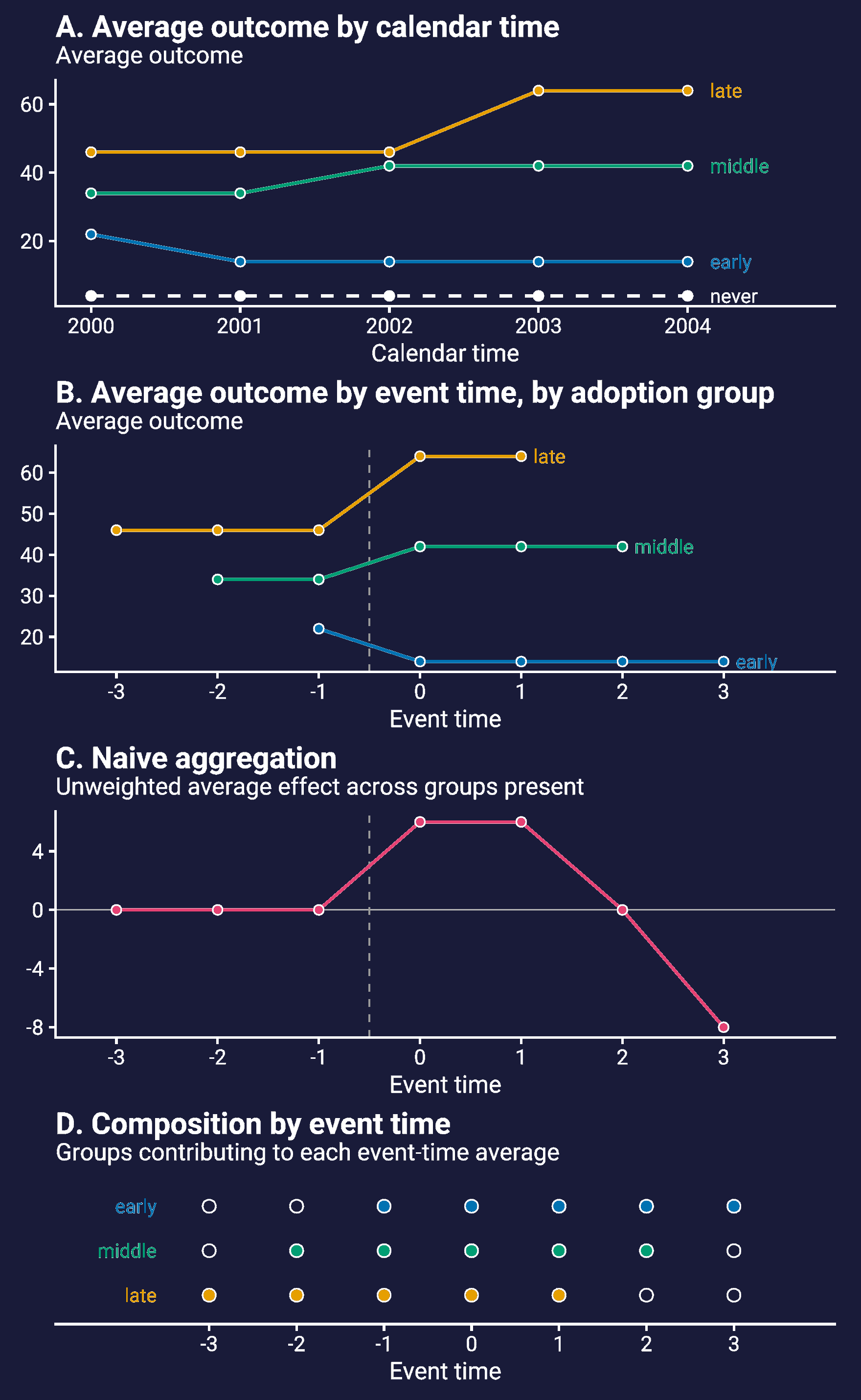
Cohorts adopt at different calendar times, so they are observed for different horizons. If you simply average every identified cohort at each event time, the set of cohorts in the average shrinks as the horizon grows: the late adopters dominate the left edge of the event-time panel and the early adopters do the same for the right side. This means the aggregate can change with event-time even when every cohort’s effect is constant.
Paper Exhibit 1, a deterministic illustration. Three cohorts (early, middle, late) adopt at different calendar times and carry constant but different effects. (A) Average outcome in calendar time. (B) The same series recentered on each cohort’s adoption date (event-time). (C) A naive aggregate that simply averages whichever cohorts are present at each event time manufactures a rise and then a fade-out — even though every cohort’s effect is constant. (D) The reason is the changing composition: which cohorts contribute to each event-time average (filled markers = present). Trimming every sub-experiment to a common event window holds that composition fixed, so a constant effect reads as constant.
Paper Exhibit 1, a deterministic illustration. Three cohorts (early, middle, late) adopt at different calendar times and carry constant but different effects. (A) Average outcome in calendar time. (B) The same series recentered on each cohort’s adoption date (event-time). (C) A naive aggregate that simply averages whichever cohorts are present at each event time manufactures a rise and then a fade-out — even though every cohort’s effect is constant. (D) The reason is the changing composition: which cohorts contribute to each event-time average (filled markers = present). Trimming every sub-experiment to a common event window holds that composition fixed, so a constant effect reads as constant.
Compositional balance is not an issue limited to stacked DiD. This can be an issue for any method. However in our case, it is especially helpful to have compositional balance as it makes the weights simpler to calculate. Therefore, we have built this into the method by requiring the user to choose \(\kappa_{\text{pre}}\) and \(\kappa_{\text{post}}\). These trim every sub-experiment to the same event window and keeps only cohorts that can fill it, so the composition is constant across event time by construction. kappa_trade_offs() shows exactly which cohorts survive each choice. This creates a user degree-of-freedom in the event-time to consider. Often you will face a trade-off between long pre/post treatment periods and broad representation of many treated groups. In practice it likely makes sense to ensure your kappa decisions are not driving your estimated effect in some undesireable way.
Imbalance across cohorts
The second kind of imbalance is between cohorts. A big cohort and a small cohort draw controls from the same pool, so their ratios of treated to control units differ — and, as the explainer shows, an unweighted stacked regression averages treated and control trends with weights driven by that ratio, not by the treated mass. The Q-weights rescale each cohort’s controls to remove the mismatch.
You can see the imbalance directly on the stack. Below, one cohort holds 80% of the treated units but only a quarter of the control pool; its control observations get upweighted (q_weight well above 1) to compensate, while the small cohorts get pulled down.
stacked use medicaid, clearstacked build, time(year) unit(state) adopt(adopt_year) kpre(3) kpost(2)* Treated vs control balance and the control Q-weight, by cohorttable sub_exp if event_time == 0, /// statistic(mean q_weight) statistic(count treat)
The 2014 cohort’s controls carry a mean weight near 2.9, while the small later cohorts sit well below 1. That is the correction at work: it is undoing the fact that the big cohort’s treated mass is under-represented in the shared control pool.
The divergence statistic D
How much can the correction actually change the answer? That is bounded by a single number you can compute from adoption dates and cohort masses alone, before any outcome is examined. D compares two weight vectors over the cohorts:
\(w_a^{S}\) — the precision weight an unweighted stacked TWFE implicitly puts on cohort \(a\);
\(w_a^{T}\) — the corrective weight the design targets (cohort \(a\)’s share of the treated mass).
When \(D \approx 0\), the unweighted and Q-weighted estimators cannot differ much no matter what the treatment effects turn out to be. When \(D\) is large, the unweighted estimate is exposed to effect heterogeneity — it can diverge sharply from the target, up to and including a change of sign. D is a statement about the design’s vulnerability, not a prediction: a large \(D\) means the two estimates can diverge, not that they must.
Compute it with the screen = TRUE option to kappa_trade_offs():
Here \(D \approx 0.31\): the design is unbalanced (the 2014 cohort dominates the treated mass). Yet on this dataset the naive and Q-weighted post-period ATTs are nearly identical (\(-0.0219\) vs \(-0.0222\)) — a reminder that \(D\) bounds the possible divergence, and the cohort effects happen to be similar enough that little of that possibility is realized. Always screen under the same masses your target uses: a design balanced in unit counts can be badly unbalanced in population, so pass the matching weight_type (and pop_var) to kappa_trade_offs().
To see what happens when \(D\) is large and the effects are heterogeneous — the case where the correction is not optional — work through the sign-flip example.